Multisim Tutorial

Introduction:

 

Multisim is a circuit simulator powered by SPICE. SPICE is the industry standard circuit simulation engine, developed here at Berkeley. SPICE itself is extremely difficult to learn and use, so programs such as Multisim provide an intuitive front end for the powerful SPICE engine. Almost any circuit can be modeled in Multisim, and the model can be tested using Multisim’s virtual lab bench which includes oscilloscopes, function generators, etc. You will learn to draw and test circuits in Multisim. Note: There is a Printed Circuit Board (PCB) program called Ultiboard 11.0 for permanent Board work available.  You do not need this but you can use it if you want for any final work.

Example:

 

Let’s try the following RC high-pass filter:

Open Multisim by clicking on Start -> Programs -> National Instruments -> Circuit Design Suite 11.0 -> Multisim 11.0 . Create a new file with File-> New-> Design.

First we need to find the components. There are a few ways: Place -> Components (Ctrl + W) or right-click a blank spot and go to Place Component. The AC source is in the “Sources” group (top left), “Signal Voltage Sources” family and is called “AC Voltage” select it and click on OK. A ghost component is now pinned to the cursor. Choose an appropriate spot and click to place the component. Components, and the associated labels, can be dragged after placement. Rotate components with Ctrl+R flip them with Alt+X and Alt+Y.

Now place the ground (hint: look in the “Power Sources” family). The ground is one of the most important components in every Multisim circuit: the mathematics of SPICE requires every circuit have a power source and a ground, or else nothing will work! Next find the capacitor, in the “Basic” group. You can either select the correct valued capacitor from the list or place one and double-click it and modify the value. Metric prefixes (or their one-letter abbreviations) can be typed in the box along with the number. 

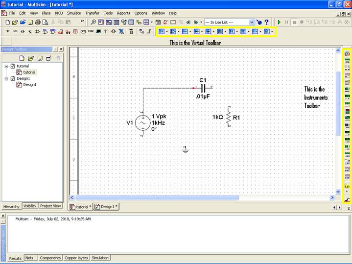
For the resistor let’s use the Virtual Toolbar (shown below) to quicken the process. (If you don’t see a toolbar with 9 blue buttons, right click any of the toolbars and check that “Virtual” is on.) Click on the “Basic” group (with a resistor icon) and choose “Place Virtual Resistor” (notice that you could have found the capacitor in the same place). Place the resistor and make sure it is the right value if it is not, double click it and change the value.

Up to now you must have something like this:

Wire the circuit by clicking on the end points of the components (do not worry about the “1” and “2”’s written on the ends of the components). If you need to make multiple connections at the same point you can add a Junction by going to Place-> Junction (Ctrl+J). You might be afraid that the connection has not been made since MultiSim does not really show a connection but as long as you click on the red dot that appears near the terminals the connection will be made. To connect a wire to a component you only need to click once near the red dot however to leave it loose you need to double click (the red dot is visible in the picture above.) A quick way to make sure a connection exist is by dragging the component and seeing whether the wire comes along.

 

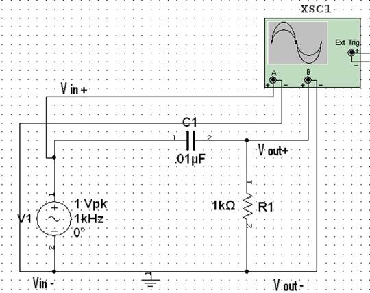
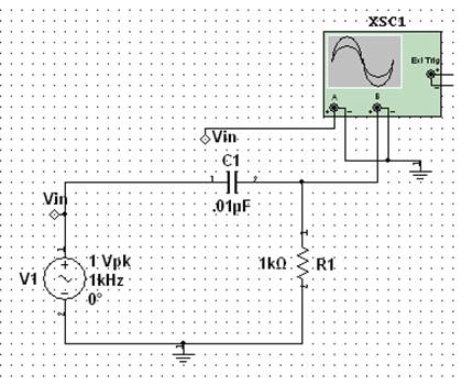
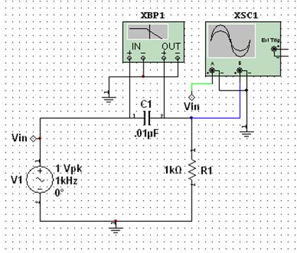
Now choose an oscilloscope from the right hand toolbar (the Instruments toolbar). You have four choices; for most circuits the generic 2-channel oscilloscope does the job.  So click on the one that is simply called “Oscilloscope” and stick it in your favorite spot on the board. Channel 1 is normally used to look at the input of the circuit, and channel 2 is used for the output. After placing the oscilloscope and wiring it to the input and output terminals it should look like (without the yellow circle):

Notice that when two wires simply pass over each other there is no connection (inside the yellow circle) but where the wires are actually connected the connection is represented by a dot. 

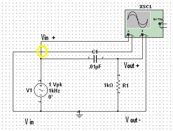
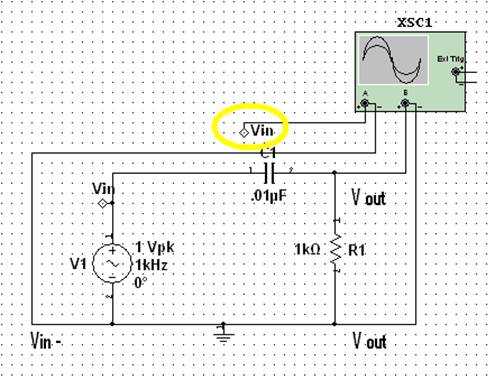
 If the wiring is messy you can use an On Page Connector (in this circuit it might be overkill but it will be useful later), to use the On Page Connector go to Place-> Connectors-> On Page Connector (or Ctrl+Alt+O). In the box that appears name the connector something useful (e.g. Vin) and place it somewhere so you can connect it to the positive side of the channel A of the oscilloscope. An On Page Connector behaves like a wire those with the same name are electrically connected so get another connector and in the window that appears double-click on the name that you chose earlier and put the connector near the positive side of the AC source as shown below.

 We can make the circuit yet a bit more organized. Since the negative inputs of the oscilloscope are connected to the ground we don’t have to have the wire go around the circuit and we can just connect these two wires to a ground closer to the scope.
 

Simulation:

 

Click the green play button in the Simulation toolbox, or click the toggle switch in the upper right corner of the page (or you could go to Simulate->Run). Double-click the oscilloscope and set the horizontal and vertical scales appropriately. The trace should look like this: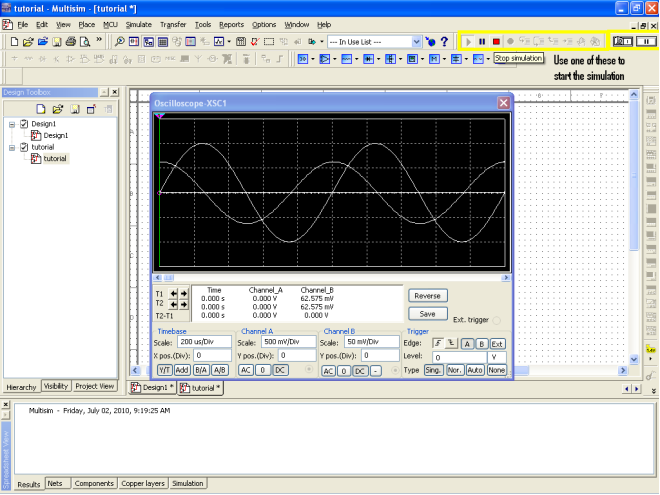

It is hard to see which graph corresponds to which input, to solve this problem, we will change the color of the wires that go into the oscilloscope and that would change the color of he graphs. To change the color of the wires right click on them and choose “Color Segment” then choose the color and click ok it is good practice to use the colors that you would have used if you were to physically set up the circuit. The new wiring might look like:

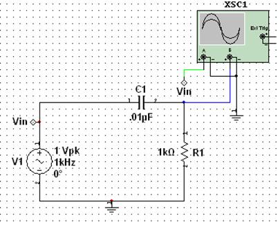
(I have pulled the oscilloscope a little to the right to make room for our next task)

 

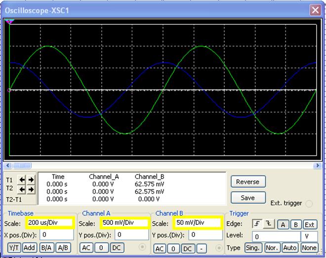
Run the simulation and double click on the oscilloscope again change the divisions to the one shown below to get a similar graph.

 

Change the input frequency (or any other parameter) on the Value page found by double-clicking the source to see their effect on the graph. Most components can be modified through the double-click menu however you must be sure that the simulation is not working because otherwise the value will not effect the circuit until you restart the simulation.

To learn more about the circuit we want to see the transfer function. If one wants to do this manually one must feed the circuit different signals and measure the response of the circuit, however, MultiSim has an instrument that does exactly that. It is called Bode Plotter. Bode plots are traditionally done in log axis and are most useful to determine the role of frequency on the circuits and as you might have found out this circuit is strongly frequency dependent. To get a bode plot, place a Bode Plotter from the instruments toolbar and wire it as shown below.

 

To make sense of the connections it might help to see the circuit from the Bode plotter’s eyes. The Bode plotter disables the AC source (to use Bode Plotter you must be sure you have an AC source in your circuit) so to the Bode plotter the above circuit and connections (without the oscilloscope) look like:

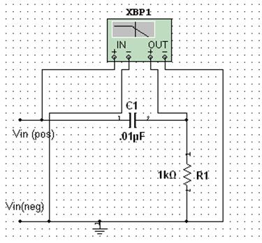
Because the V- are connected to the ground it makes the wiring more organized if you just place a ground near the plotter and connect the circuit to it.

Double click on the bode plotter. You should see a figure similar to the following figure.

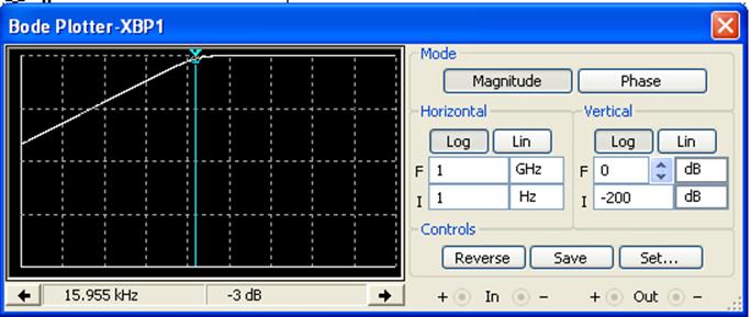
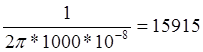
The bode plot is especially useful because it helps us determine the cutoff frequency of the filter. To do so drag the cyan cursor to the top left of the plot to -3 dB or right click on it choose “set Y value =>” and type in -3 then the frequency will represent the roll off frequency of  the circuit. The bode plot tells us that the frequency is about 15.955 you should be getting the same value if you used the same components. Using the formula we get:

 = not bad at all!

You can also see the phase change caused by the circuit if you click on phase button.

Analysis:

 

There are many types of analysis that are easy in Multisim. Let’s find the transfer function again, to check our results. Go to Simulate-> Analyses->AC Analysis and make sure everything is set how you want.

 

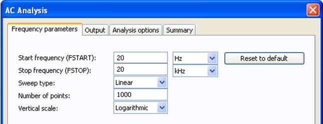
Now look at the output tab. You must add any quantity that you want to analyze. If you don’t recognize the variables you want, rename them. Cancel the analysis and double-click on any wire you want to monitor. Type something related for the Preferred Net Name field (e.g. Vout).

When the analysis is finished Grapher automatically opens. Your analysis results should look something like:

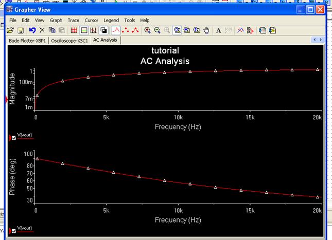
The scales of any axis can be changed, along with other properties, by right-clicking the axis and selecting Properties. You may also use the toolbar at the top to navigate the graphs.

            You’ll notice that the information displayed on any instrument in your schematic shows up on separate tabs in the Grapher window. To see Grapher without running an analysis, go to View-> Grapher. Old graphs can be deleted by clicking the “X” in the top toolbar, next to the Undo button, twice.

And a final note: for non-periodic or unusual waveforms, use the PWL (Piecewise Linear) Source.