Lab 1 - Introductory Experiments and Linear Circuits I
University of California at Berkeley
Donald A. Glaser Physics 111A
Instrumentation Laboratory
Lab 1
Introductory Experiments and Linear Circuits I
© 2016 by the Regents of the University of California. All rights reserved.
General guidelines:
-
Always read the entire Lab Writeup before coming to lab. Lab time is precious. Don't waste it reading the background material.
-
Likewise, do the pre-lab questions before you come to lab. You are required to do the prelab questions before beginning benchwork. Information required to answer the prelab questions can be found in the background material at the beginning of the lab, from lecture, in the stated references, and on the web.
- As best you can, formulate a plan to perform the Lab exercises.
- Please ask questions of the GSIs or Professor if you don't understand something (or you think you know something that we don't) at any time during the course!
- Please clean your work station at the end of class or when you leave. Resort all the prestripped wires, return your components to the proper drawers, place your bnc jacks, minigrabbers, 50 ohm terminators, Tees, etc, back in their box, and neaten all your BNC cables.
Note that you can check out and permanently keep one (per person) portable breadboard, VB-106 or VB-108, from the 111-Lab . Store these breadboards in the shelves along the west wall. As you build more complicated circuits, you will find it useful to keep your circuits assembled on these portable boards until you next class. You must disassemble circuits on lab station breadboards. - Wikipedia has many useful and informative articles.
- Reprints and other information can be found on the Physics 111 Library Site.
Important safety habits:
- When you are done for the day, make sure you power down all equipment.
- Never place food or drink next to any apparatus. Accidental spills can damage or destroy the equipment and your experiment and give you a shock. Food can only be consumed on the designated, marked tables.
This lab is unusual in that it has two parts. In your prelab prep, concentrate on the Part 1 before your first lab day, and Part 2 when you have complete Part 1. You do not need to have completed the Part 2 prelab questions before beginning Part 1.
Part 1 of this lab introduces you to the equipment you will be using throughout the 111a lab and most of the labs in Physics 111b, particularly the digital multimeter (DMM), breadboard, power supplies, oscilloscope, and the signal generator. The breadboard, power supplies and some other components are integrated into a box found at each lab station.
Everyone needs to have a working knowledge of this equipment before continuing with the rest of the 111a course. Note that the manuals for the lab equipment are posted online. The XYZ’s of scopes contains a general introduction to oscilloscopes.
In Part 2 of this lab you will study circuits made from linear components such as resistors, and capacitors. You will build filters and learn the concept of frequency dependent impedance and its importance in circuit analysis and electrical measurements. You will also learn why we use scope probes and terminators for scope measurements.
|
"Student Manual for Art of Electronics", Hayes & Horowitz |
Chapter 1, p 1–31 and p 32–60 |
|
Horowitz & Hill, 3rd edition |
Chapter 1.1–1.4, 1.7 and Appendixes A, B, C, D, skim H, and O. (You'll read the rest of Ch. 1 for the next two weeks, so you might want to get started now.) |
| Look at other Books available | Readings |
All parts spec sheets are on the Physics 111 Library site.
Note that you can generally find most of the information that you need for the labs in the lab writeups themselves. The references listed above are for background and more in depth explanations.
Legend for the lab writeup symbols
 This problem should be done before coming to the 111 lab.
 This problem must be checked and signed off by the GSIs or the Professor. You may continue on to your next question while waiting for a signoff, but keep your setup for the signoff question.
Pre-lab Questions:
Pre-lab questions (Part 1):
1. Write a short paragraph each explaining how the breadboard, power supply, multimeter, oscilloscope, and the signal/pulse generator are used.
2. What is the difference between the common and the ground of a circuit?
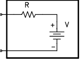
3. Derive the voltage divider equation ( $\frac{V_{out}}{V_{in}}=\frac{R_2}{R_2+R_1}$) for the following circuit:
Pre-lab questions (Part 2):
1. What is impedance? Input impedance? Output impedance?
2. What are the interesting properties of a coaxial cable and transmission lines? (hint: Wikipedia.org)
3. What is a low-pass circuit? A high pass circuit? Draw an example of each. Derive the transfer function for each of these circuits.
Now let’s play with the equipment. video link introduction below;
Keithley 2110 Digital Multimeter (DMM)
|
|
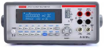
The DMM is used to measure voltages, currents, resistances and several other more complicated quantities. The DMM is a relatively simple instrument.
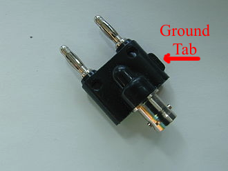
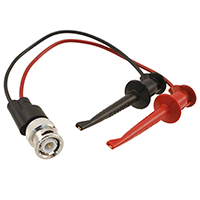
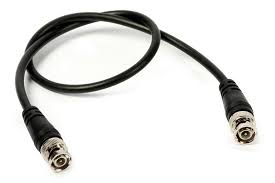
Turn on the digital multimeter by pressing the power button located to the left on the front panel. To make a measurement with the DMM, first connect a double banana plug to one end of a BNC cable and a pair of mini-grabbers to the other end. The outer shield of the BNC is traditionally at ground; the inner wire carries the signals. When the BNC cable is attached to a double banana plug, one of the plugs will be attached to the outer shield, i.e. the ground, and the other to the signal. Figure out which of the banana plugs is labeled ground. Look for the little black tab on the banana plug pair; this tab will the ground.
| Double Banana Plug | minigrabber | BNC Cable |
 |
 |
 |
Voltage
Find the pair of red and black inputs on the DMM that indicate where to insert the banana plugs to make a voltage measurement; remember that red is positive and black is ground and hook up the banana plug accordingly. You have two different voltage measuring options: DCV and ACV. DCV measures voltage created by a DC current and ACV for an AC current. You can change the DMM’s range to maximize your measurement’s resolution by pressing the up and down arrows labeled “Range +” and “Range – “.
Resistance
Be sure to disconnect the electronics component you wish to measure from the circuit before making the resistance measurement (think about why it is better to do so). You also have two options for measuring resistance. One is the standard 2 wire measurement and the other is a 4 wire measurement. The 4 wire measurement method is used for measuring very small resistances when even the resistance in the copper wire leads is important. Because this lab won’t be dealing with such low resistances, the majority of the measurements you make will be done with the standard 2 wire method. To make the measurement, hook up the banana plug to the correct red/black inputs for measuring resistance, indicated by the \(\Omega\) symbol, and select the 2 wire resistance option indicated by the \(\Omega^2\) symbol.
Capacitance
Same setup as the voltage and resistance measurements. The capacitance measurement option is indicated by the capacitor symbol.
Current
Current measurements also have two options: DCI and ACI. DC current measurements using this DMM are tricky because the appropriate jacks, the black jack on the right and the white jack on the left, are too far apart to have a single banana plug inserted into them. To compensate for this problem, we will be using two banana plugs and only use the center conducting wire of two different BNC cables to perform the measurement. Consult the picture below for how this is done.
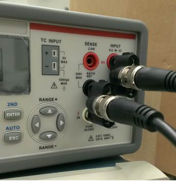

Here we are measuring the current flowing across a resistor. Notice how the banana plugs are inserted in and how we are only using the red grabbers, or the center conducting wires, to make the measurement. Conversely, we could flip the orientation of both banana plugs and only use the grounding (black) wires to make the measurements instead. The important thing to note is that any DC current measurement requires the left white jack and the right black jack to work; you can insert the banana plugs in any orientation you want but you must remember to use the correct BNC grounding or conducting wires.
ACI measurements are easy because we only need one banana plug. The jacks for an ACI measurement are the black and white jacks on the right. Be sure to hook up the banana plug with the correct polarity.
Alternate method to measure current:
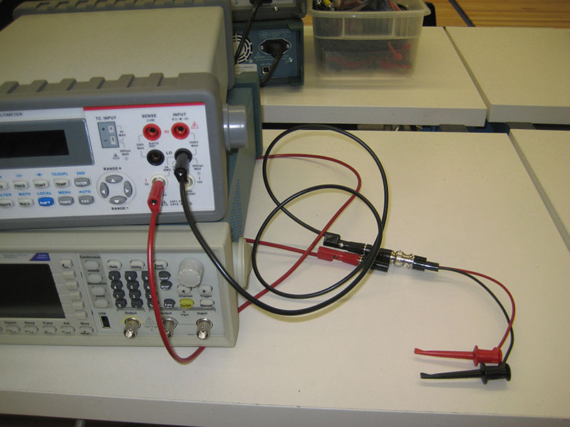 DMM Hookup connections for current measement DMM Hookup connections for current measement |
 Note black and red leads are in series with the resistor to measure current. Note black and red leads are in series with the resistor to measure current. |
Connect the DMM leads in parallel with a component to measure voltages across it, and in series with a component to measure currents through it. When measuring the resistance of a component, the element must be isolated from the rest of the circuit.
Video link introduction above;
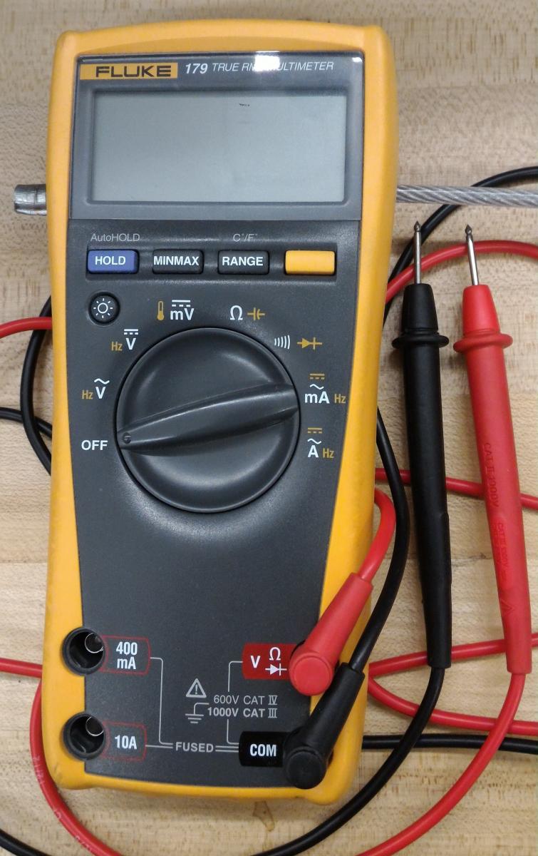 The Fluke meter is similar to the Keithley, but less accurate. It is good for quickly measuring voltages and resistances. On the
  setting, the DMM will beep when there is a low resistance path between the two leads; this "continuity check" setting is used to trace wires paths.
Breadboard Box
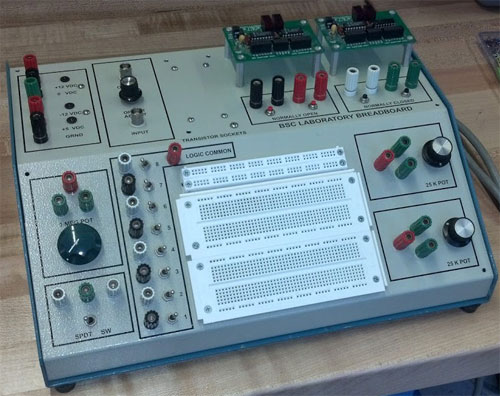
(B) BSC Laboratory Breadboard Box
Breadboard
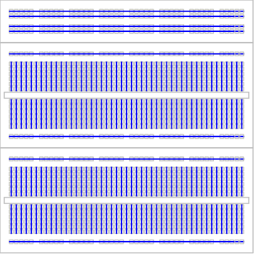
Commercial electronic equipment is constructed on printed circuit boards; “wires” are photo-etched onto a sheet of copper, and components are soldered into place. To save time and effort, we will build our prototype circuits on solderless breadboards. A breadboard is an insulating board with a regular pattern of holes that can be used as sockets. The sockets are interconnected with hidden wires, and electronic component leads or wires pushed into the socket holes will make contact with the interconnecting wires below. The interconnecting wires on our breadboards follow the pattern shown by the heavy lines in the drawing below; the gray squares indicate the positions of the sockets.
|
Figure 1: Breadboard |
Breadboard Practice:
Use 22-gauge solid (not stranded) wire to make connections. [Wire gauges (thicknesses) are listed at https://en.wikipedia.org/wiki/American_wire_gauge.)] Use the precut wires, or, for long runs, cut interconnecting wires to the right length. Strip ~3/8” of insulation from each end, and poke the bare wires into the breadboard socket holes until they bottom out. The breadboards are delicate! Forcing wires or component leads into the board can damage the sockets or make a poor connection. Wires or leads that do not fit easily into the breadboards may be too thick.
· Use the buses (the long horizontal strips shown in Figure 1) for power and ground connections. Good bus habits will save you lots of time and trouble with complicated circuits by making your circuit wiring more transparent and by removing unnecessary clutter.
· Build your circuits compactly. Long leads between components introduce stray capacitance and can result in oscillations or high frequency [e.g., radio frequency (RF)] pickup.
· For clarity, signals should flow from left to right; place input signals on the left side of the board, circuitry in the middle, and output signals on the right side.
· Use color-coding to make your wiring clear: by convention, red wires are used for power connections, black wires are used for ground connections, and other color wires used for signals. Following this convention, espcially for the long wires that you cut yourself, will help enormously when working with complex circuits later in this course.
Problem 1.1.1 - Breadboard Layout
Use the Digital Multimeter (DMM) in resistance-measuring mode to check some of the internal connections in the breadboard. Make sure you understand how the breadboard is set-up: what is connected and what is not. Sketch a simple diagram showing what connects where on the breadboard. Your sketch should suffice to explain the breadboard to someone using it for the first time.
Commons and Grounds
Recall that voltage is a measure of the potential difference between two points. Although we say “the voltage at point A”, we really mean “the voltage at point A with respect to the local zero-potential reference point.”
|
The most useful zero-potential reference point is the earth itself—the “ground.” A ground in any circuit is defined to be any wire, lead or bus somehow connected to the earth. The power company thoughtfully provides a wire connected to the earth in all three-pronged power outlets, and that ground wire is often connected to a ground lead in electrical equipment. Thus, the potential of a point in a grounded circuit is the same as the potential difference between that point and the earth. Why do most electrical wall sockets have three leads? The electric company intends current to flow between the hot and neutral wires in the wall socket, the two rectangular slots. No current should flow in the ground wire. The electrical company arranges its transformers so that the hot lead is approximately 120V from the neutral, and the neutral is approximately at ground. But things are rarely perfect, and the neutral lead is often a few volts from ground. As for the ground lead itself (the horseshoe shaped hole), the electric company grounds the lead by actually attaching it to a long conducting rod stuck into the earth. Look for the ground wire the next time you walk by a transformer on a pole! Other good grounds are available. Cold water pipes, for example, are well connected to the earth, and are often used as grounds. The electric company doesn’t supply the ground as a courtesy for electronic circuits builders; they supply it for shock prevention. Electrical shocks occur when a sufficiently high voltage drives a sufficiently high current through the victim’s body. Most dangerous are shocks in which currents travels through the victim’s heart; only 50mA can be lethal. Grounding the outer case of a piece of equipment greatly reduces the chance of shocks by shielding the user from any high internal voltages. It is difficult (but not impossible!) to get a serious shock with voltages less than about 50V. While you should always think before touching a bare wire, shocks should not be a problem with any of the circuits in the BSC lab. Caution: Standard electronic circuit construction always uses black for ground, red for power and other colors for signal leads. BUT North American building wiring always uses white for neutral, BLACK FOR HOT (the dangerous lead) and green for ground.
|
 |
|
North American Power Outlet |
While grounding a circuit is usually beneficial, it is not actually necessary. Cell phones, for instance, are not grounded. For these circuits we define a “common” for the voltage—a local point that all measurements on the circuit refer to.
Power supply
 |
Red |
+12V |
|
|
Black |
0V |
||
|
Green |
-12V |
||
|
Red |
+5V |
||
|
Black |
0V |
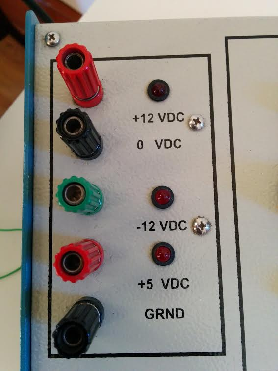
Each station has two power supplies built into the box carrying the breadboard. The first supply (bottom two terminals) has an output voltage of 5 V and is used mainly with digital circuits. The common of the 5V supply is marked 0V, and is connected to the metal chassis of the breadboard box, which is in turn connected to ground. Thus the common of the 5V supply is also a ground.
The other supply, the top three terminals, supplies 12V between adjacent terminals. This power supply “floats”, i.e. it is not connected to ground. A floating supply maintains its rated voltage difference between its terminals, but its absolute potential can float up or down. Usually ground is attached to the 0V terminal, but it may be useful to attach it to either of the other two terminals. Watch out: leaving the power supply floating, or inappropriately grounding the supply, can lead to subtle circuit failures. If you use both the 5V and the ±12V power supplies in a circuit, make sure that the ±12V supply is referenced to the 5V supply.
Note that the voltages labeled ±12V are actually closer to ±13.1V, but throughout this class we will refer to them by their nominal value, namely as the ±12V supplies.
|
Problem 1.1.2 - Power Supply Voltages: Conceptual
How should you hook up the power supplies to get the following voltages with respect to ground:
a) +24V, b) –24V, c) +12V, d) –12V, e) +17V? Sketch a simple diagram for each one. Remember that ground is a zero voltage point reference. |
|
|
Problem 1.1.3 - Power Supply Voltages: Measurements Setup, measure, and record the power supply voltages required in Problem 1.1.2. What does the DMM read when you measure the potential between the +12V output and 5V supply ground (the GND terminal) if you don’t hook up any other wires? Explain why you don't measure 12V! Remember to turn on your supplies with the switch on the side. All three lights should glow. |
The following Breadboard Box components will be occasionally useful throughout this semester. For now, read the descriptions and locate these components on the Breadboard Box, but there are no exercises that require them in this lab.
|
Offset Adder |
|
Buttons and Switches |
|||
|
The Offset Adder adds a constant voltage to the input signal. The constant voltage can be adjusted by turning the Offset Adjust knob, and can be either positive or negative. |
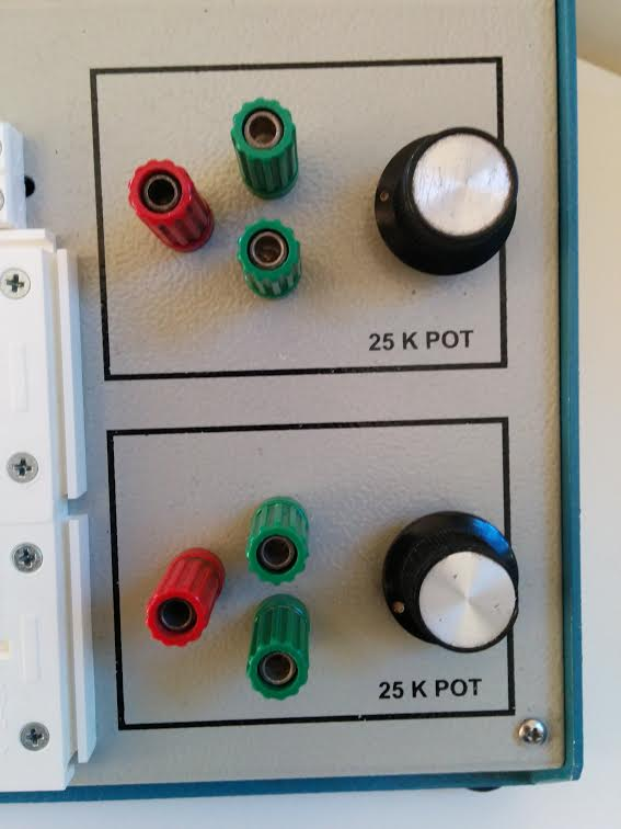
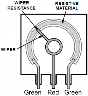
There are two 25k and one 1M potentiometers on the breadboard. Potentiometers are resistors whose resitance can be varied. Potentiometers have three terminals; turning the knob changes the resistance between the red terminal, called the wiper, and the green terminals. The resistance between the red terminal and one of the green terminals will vary from 0 to the designated resistance, while the resistance between the red terminal and the other green terminal varies inversely, i.e. between the designated resitance and 0. The resistance between the two green terminals is constant at the designated resistance. |
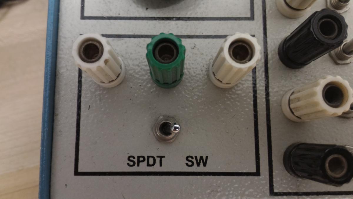
There are two normally open buttons, two normally closed buttons, and one SPDT switch on the Breadboard Box. Normally open means the circuit is open until pressing the button closes (shorts) it. Normally closed means exactly the opposite; pressing the button opens it. The SPDT (single-poll double-throw) connects the green terminal to the left white terminal when the switch is to the left, and to the right white terminal when the switch is to the right. |

|
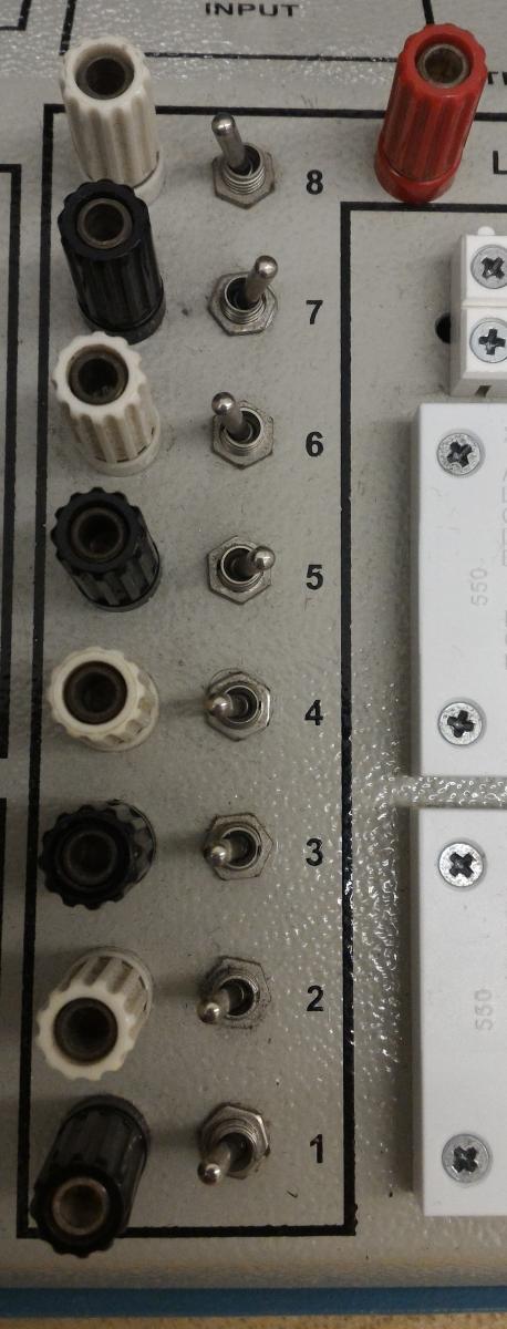
Logic Switches
|
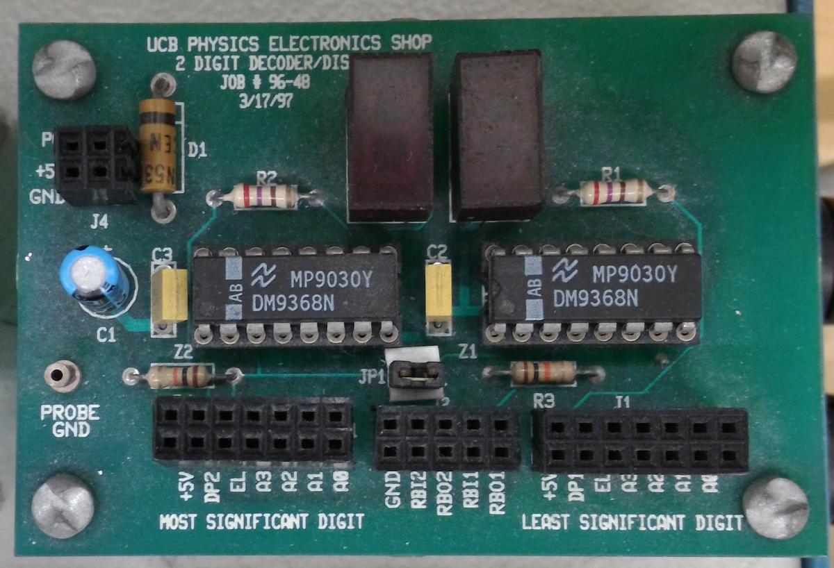
Printed Circuit Boards (PCB) |
|
| The eight logic switches are all referenced to a single logic common. Throwing the switch puts it in either a HIGH or LOW state. These can be connected to a circuit to easily switch the voltage from high to low or vice versa. | There are two PCBs on the breadboard. These boards contain digit displays that are no longer commonly used in this class. Each PCB has two 9368 chips and two FND357 chips along with various other components. The displays are wired as specified in the silkscreen text at the PCB bottom. |
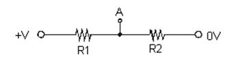
Problem 1.1.4 - Voltage Divider: General Calculation
|
Calculate the voltage at point A with respect to 0V in the general case shown here. You will use this “voltage divider” formula in every lab in the course!
|
 Problem 1.1.5 - Voltage Divider: Specific Current Calculation
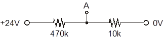
Now calculate the current through each resistor using the specific values shown in the schematic at right. Show the circuit and calculations in your notes. Note that the ohm symbol $(\Omega)$ is traditionally suppressed when showing resistor values in a circuit diagram. Hence, the label "470k" means a resistor with value 470 $\mathrm{k}\Omega,$ and 10k means a resistor with value 10 $\mathrm{k}\Omega$. A circuit label of 330 next to a resistor would be 330$\Omega$.
Problem 1.1.6 - Voltage Divider: Specific Voltage Calculation | Calculate the voltage at point A with respect to 0V for the circuit values above and the formula you derived in 1.1.4. |
Problem 1.1.7 - Voltage Divider: Measurement Setup
| How should you connect the DMM in order to measure a) the current through the 10k resistor, b) the voltage drop across the 470k resistor? Sketch the corresponding circuit diagrams for each of these measurements, showing the connections to the DMM. |
Problem 1.1.8 - Voltage Divider: Component Measurements
Obtain the 10k and 470k resistors necessary to build the divider in problem 1.1.5 from the resistor stock on the West wall. Resistors are often misfiled. Always check the value of the resister by reading its color code, given by the colored bands printed on the resistor. The resistor color code is posted in the lab near the resistor stock, and can be found at https://en.wikipedia.org/wiki/Electronic_color_code.
Even if you have obtained the correct resistor, it will not have precisely the value that you desired. Actual component values vary around their specified values; a 10k resistor is never exactly 10k. The specified values, as opposed to the actual values, are often called the "nominal" values. With the DMM, measure and record the actual values of these resistors.
The tolerance for most of the resistors in the lab is ±5%. This means that the measured value of the resistor should be within ±5% of its nominal value.
Do the measured and nominal resistances agree within the specified tolerance?
Repeat the calculations of Question 1.1.5 and 1.1.6 using the actual measured resistances and voltages rather than the nominal ones. Note the difference between these calcualted values and the nominal calculated values.
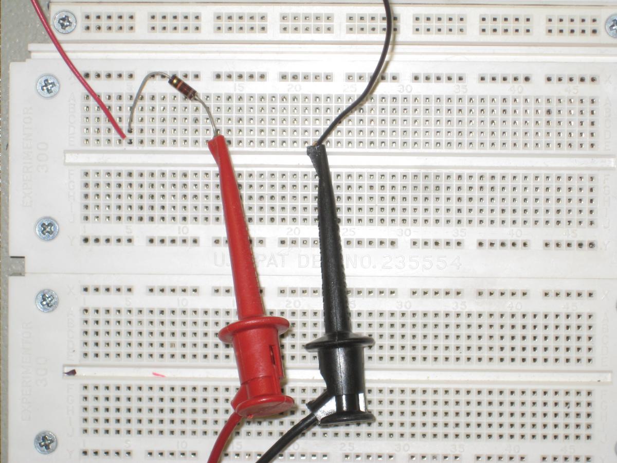
Now use the breadboard, the power supplies and the DMM to build the voltage divider pictured above with your 470k and 10k resistors. Your circuit should look something like the pictures below.


Measure the voltage at point A as precisely as possible. Note that this is one of the few times in this course when you should write down many significant figures. Bench electronics is generally a 10% science.
Estimate the error (uncertainty) using the example below, which comes from the Kiethley DMM manual:
Accuracy (error) = 0.012% of value + 0.004% of range (i.e. 1mV, 10mV, 10 volts)
As an example of how to calculate the actual reading limits, assume that you are measuring 5V on the 10V range.
Accuracy = 0.012% of value + 0.004% of range
0.012% * 5 V + 0.004% * 10 V
0.0006 V + 0.0004 V
0.0010 V
Thus, the actual reading range is 5 V ± 1 mV or from 4.999 V to 5.001 V.
DC current, AC voltage, AC current, and resistance errors calculations are performed in a similar manner using the pertinent specifications, ranges, and input signal values.
Does the voltage at point A agree with the value calculated in Section 1.1.9? Comment on the closeness of your calculated and measured values. Do they agree to within the measurement uncertainty?
Problem 1.1.11 - Voltage Divider: Current Measurement
Measure the current through the resistors. Is your result consistent with the calculated values? (Specify your measurement's uncertainty.)
Problem 1.1.12 - Voltage Divider: Power Calculations
|
Using the nominal values for simplicity: a) Calculate how much power each resistor dissipates. Are your resistors rated for this power? (Hint: these are 1/4 watt resistors.) b) Keeping the same 24V supply and keeping the ratio of the resistors the same, would you increase or decrease the resistor values to approach the maximum power rating of the resistors? c) If you were to change the resistors as suggested in b), which resistor would reach its max power rating first? d) Calculate how much larger or smaller (5 times smaller? 100 larger?) you would have to make the resistor values until one resistor first exceeded its maximum power rating. |
Tektronix MSO 2024 Digital Oscilloscope
Video link introduction above; Spec sheet PDF
The oscilloscope is the most important instrument in any electronics lab, as well as in many physics labs. To do well in this lab and in 111b you must be fluent with its operation.
|
"Scopes" are used to take a picture of a signal — a time-history or “scope trace” of the amplitude of the signal. The trace moves horizontally, from left to right, across the screen at a fixed, but adjustable rate, drawing the amplitude of the signal vertically. When the trace comes to the end of the screen, it jumps back to the beginning at the left. Usually, the trace moves horizontally so fast that you can't see its progress across the screen, but a slow (low frequency) signal is shown at the right.
|
|
| Triggered Scope Displaying a Slow Signal |

|
Most, but not all signals, are repetitive. If this is the case, succesive traces may overlay, and potentially, we may be able to see a quasi-static image like that shown at right. |
 |
|
Triggered Scope Displaying a Fast Signal: Note that the signals overlay.Traqce |
|
Trace image overlay will only happen if the time it takes the trace to move across the screen is an integer multiple of the period of the waveform being viewed. This is a rare. Normally, this doesn't happen, and one gets traces that look like those shown at right. Notice how the phase of the signal jumps around. With normal trace draw speeds, this signal would be completely jumbled as numerous traces would be overlaid with random start phases. To stop this from happening, scopes are "triggered". Before each trace starts from the left, the scope waits until the signal reaches a specified amplitude. Only when the signal reaches this amplitude does the trace begin. This will align the scope traces at the same phase, and we will see the desired quasi-static image. Scope triggering is tricky and frustrating...it is probably the most difficult thing about using a scope. With practice, you will get good at it. |
 |
| Improperly Triggered Scope |
A scope is a very complicated instruments. The 111a scopes have over sixty controls…and these are relatively simple scopes. Fortunately most of these controls are rarely or never adjusted while taking routine measurements; only a four controls determine the scope’s basic operation. These primary controls are indicated on the panel drawn below.
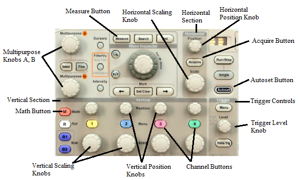
The four important controls, which will be discussed in more detail later, are:
- The Vertical Scaling Knob adjusts the vertical size of the image on the scope screen; a typical setting would be 1V/div.
- The Vertical Position Knobs move the scope traces up and down.
- The Horizontal Scaling Knob adjusts how fast the scope draws the image across the screen; a typical setting would be 1ms/div.
- The Trigger Level Knob adjusts the triggering voltage.
The signal itself is connected to one of the input BNC jacks on the scope. Our scopes have four channels, and can display up to four signals simultaneously.
Turning on the scope
The power button is located on the front in the lower left hand corner. The scope will take some time to start up it has a computer processor; do not press any buttons during this time.
Viewing an electronic signal
Using a BNC cable, connect the signal to one of the channels on the scope. The channels are located in the front on the bottom right of the scope and are labeled “1, 2, 3, and 4”.
Do not plug the signal into the “Aux In”; the use for this input will be discussed later. After you hook up the signal to the scope, you should see a trace of it appear on the screen. If you do not, play around with the scope’s viewing controls.
Vertical and Horizontal Scaling and Position Controls
The vertical scale for each of the scope’s channels is set with the knobs labeled “Scale” in the Vertical section of the scope controls and has units of volts/division. The horizontal scale for all of the channels is set similarly in the Horizontal section of the scope controls and has units of seconds/division. For example, a 100Hz 10 volt peak to peak triangle wave will take up two divisions on the 5V/division scale and one period will take up 10 divisions on the 1 ms/division scale. The current value of the vertical and horizontal scales is displayed at the bottom of the scope’s screen.
You can also adjust the position of the signal on the screen with the position controls. These are the smaller sized knobs located in the Vertical and Horizontal sections of the scope controls. The arrows on the left side of the screen indicate where ground is for each channel.
XY mode can be accessed by pressing the “Acquire” button in the Horizontal section of the scope controls and then turning on the “XY Display” option. XY mode will display two signals at the same time, the amplitude of one of the signals will make up the x-axis and the amplitude of the other will make up the y-axis. Consequently, if you put an equal amplitude sine wave as the y-axis and cosine wave as the x-axis, in XY mode the resulting trace would be a circle.
The sec/div (time-base) knob is the primary horizontal control, and controls the rate at which the scope trace sweeps (from left to right) across the screen. A scope trace of a 1ms period sine wave, displayed on the 0.5ms/div scale, would show five complete cycles of the wave.
Try this exercise: turn on the power switch, set the trigger to AUTO, to CH1, and both channel’s input switches (AC GND DC) to ground (GND). Set the horizontal time-base to 0.1ms/div. Move the vertical "position" knob slowly for channel 1 until you obtain a line at the center of the screen. Adjust the "focus" and "intensity if needed." Now slow the time-base to 0.1s/div. See how the trace sweeps across the screen?
Look at the scope's "TRIGGER" section. The "trigger circuit" determines when the scope starts its horizontal display sweep, but it needs an input. The source for this input is set by the position of the TRIGGER SOURCE switch, and the operating mode by the “A TRIGGER” switch. Look up what each switch does.
One other control deserves special mention: the Autoset button. If you cannot find the scope trace, just push this button and the trace will be pulled onto the screen and set to the correct voltage setting.

Individual Channel Configuration
You can turn individual channels on/off for viewing by pressing the corresponding channel buttons which are color coded yellow, blue, magenta and green. The menu for each channel is also accessed through these same buttons. In the menu you can configure an individual channel’s coupling, bandwidth, label, etc. To exit out of the menu, press the “Menu Off” button. (Note: A common mistake is to measure the amplitude of a low frequency signal with the channel on AC coupling. AC coupling is mainly used to measure small AC signals on top of large DC signals. Always use DC coupling unless there is a specific reason to use AC coupling.)
Triggering
Triggering on the scope will be one of the more difficult controls to understand. Recall that the scope displays a trace of the signal by constantly redrawing the signal on top of itself. The scope does this by selecting a certain amplitude for the signal to reach and once the signal reaches that amplitude the scope begins drawing the signal trace from left to right on the screen. If the signal is periodic, then the scope produces the same trace every time it draws. If the scope had selected random points along the signal to begin drawing, the resulting image would be a smear of all the differently timed traces. As a result, the scope needs to be “synched” to produce a readable signal which can be done with the trigger controls located to the far right of the scope controls.
The triggering circuit needs to know at what amplitude the signal needs to reach to begin drawing. This can be set with the “level” knob; an arrow on the right of the screen indicates the trigger level. Additionally, it needs to know which signal it is using to trigger, a.k.a. the “source”, and it must know whether to trigger when the signal has an increasing or decreasing slope. Other features include the triggering coupling, the mode, type, etc. which can all be configured in the trigger menu.
Furthermore, the scope does not need to rely on the input signal itself to tell it when to trigger. It can accept an auxiliary signal to tell it when to trigger instead. This auxiliary signal is fed into the “Aux In” channel and the source must be set to “Aux” in the trigger menu. With these settings the scope will begin drawing the trace whenever the auxiliary source triggers the scope to do so.
Making Measurements
The digital oscilloscope is capable of making measurements of the input signals such as measuring the frequency. You can configure the scope to perform a measurement by pressing the “Measure” button at the top of the scope controls. From there, select “Add Measurement” and then use the multipurpose A knob (located to right of the screen) to indicate the measurement type and the source. Afterwards, select “OK Add Measurement” and the scope will continuously perform the measurement and display the result at the bottom of the screen.
Other mathematical operations on the signals can be accessed by pressing the red “Math” button. Selecting the “Dual Wfm Math” option lets you add, subtract, or multiply two signals. The “FFT” option performs a Fourier transform. The data used to perform the transform is less than one screen width of the signal and the range can be viewed by turning on the “Gating Indicators” in the “FFT” menu; use the horizontal position control to move the boundaries over the region of the signal you want the transform to be performed. The horizontal scaling (in units of Hz/division) of the transform is indicated in the “FFT” menu to the right of the screen and can be adjusted using the multipurpose B knob.
Helpful tips for when you can’t get a good signal trace
- Sometimes the signal you see may be ridiculously larger than expected due to the “Probe Setup” being configured to “10X” which multiplies the signal seen on the scope trace by a factor of 10. Access the menu for that channel and take a look at the “Probe Setup” option to see if it is set to “10X” and change it accordingly using the Multipurpose A knob.
- If you have accidentally changed one of the settings on the scope which messed up the signal trace and do not know how to reset it, you can always return the scope to its default settings by pressing the “Default Setup” button located below the scope screen.
- If you have been playing around with the viewing controls for a while and cannot get a clear trace to appear on the screen, then press the “Autoset” button located above the Trigger controls. This will have the scope configure itself to what it thinks are the best settings for viewing the signal. (Note: The “Autoset” settings may not always be the best settings to use. Use Autoset to first get a readable signal on the screen and from there configure the viewing controls yourself to improve the trace further.)
- More information on the scope’s controls can be found on the scope's online manual. and from "The XYZ's of Using a Scope," also posted on the course website.
Problem 1.1.13 - Scope Practice
 Connect a BNC cable from the T1 output (a 1 kHz sine wave) on the Signal Distribution Box (Shown at right) to channel 1 on the scope. Connect a second BNC cable from the T2 output (a 2kHz triangle wave) to channel 2. Adjust the scope so that the image on the scope is similar to the image below (the signal amplitudes may be different.). Connect a BNC cable from the T1 output (a 1 kHz sine wave) on the Signal Distribution Box (Shown at right) to channel 1 on the scope. Connect a second BNC cable from the T2 output (a 2kHz triangle wave) to channel 2. Adjust the scope so that the image on the scope is similar to the image below (the signal amplitudes may be different.).
Practice this several times; take turns with your partner - one scrambling the controls of the scope - and the other recovering the signal. When you are ready, a GSI will scramble the controls and sign you off when you recover the signal. You do not need to write anything down. 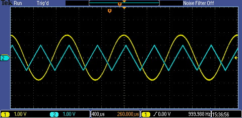 |
Tektronix AFG2021 Arbitrary Waveform Function Generator Video introduction
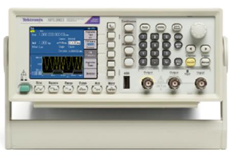
Turn on the function generator
The power button is the green button located in the lower left hand corner on the front. Like the scope, the function generator will take some time to start up; do not press any buttons during this time.
Configuring a continuous wave signal
To output a waveform, begin by selecting one of the six available waveform types using the buttons under the screen. Next, be sure that the “Continuous” button is turned on if you want to produce a pure, unmodulated waveform of the appropriate type. The current attributes of the waveform are displayed on the screen.
To change the attributes, do as follows: press the back button, the button with the arrow located to the left of the “Continuous” button, until the menu on the right side of the screen shows the options: “Frequency/Period/Phase Menu”, “Amplitude/Level Menu”, etc. Then, select the appropriate menu and the attribute you wish to adjust. You can also use the knob on the right instead of the number pad to change the attribute’s value and the right/left arrow beneath the knob to select which digit to change.
To see the signal, connect a BNC cable between the output of the function generator (the leftmost channel output BNC jack on the generator) and the scope. Turn on the channel on/off button to enable the signal. The other output is the trigger or “sync” output which produces pulses with the same frequency as the output waveform for scope trigger/synchronization purposes.
|
You may find that the signal observed on the scope has twice the amplitude of the signal that you requested from the function generator. This happens because of an impedance mismatch. There are two ways to cure this problem; use either:
Conversely, you may find the scope amplitude is half of what you requested. Either:
In summary: either you should have a 50$\Omega$terminator and have the picked the 50$\Omega$ Load Impedance option, or you should not use a terminator and pick the High Z Load Impedance option. Both configurations have advantages and disadvantages; the proper choice is complicated. Generally, you should not use the 50$\Omega$ terminator and Load Impedance configuration for signals that are below 10MHz, i.e. the vast majority of signals used in this lab. Note that changing the Ouput Menu setting does not change anything about the internal circuitry of the signal generator; it just changes the output signal amplitude listed on the generator screen to anticipate the load placed on the signal generator. Thus, if you change the Outout setting, the actual amplitude of the signal put out by the generator will not change, but the screen amplitude will immediately change appropriately. |
||
| Configuring Signal Generator Output Impedance | ||
|

Helpful Tips
Why does my function generator's output voltage not match my scope's reading.
Some of the menus are not fully displayed on the screen so be sure to check the bottom right portion of the screen to see if there is a “more” option which will let you access the rest of the menu.
Warning: When hooking up the function generator, make sure that you confirm the connections before you attach the generator to your circuit. You can burn out the generator if you attach the output of the generator to another voltage souce (like the power supplies.)
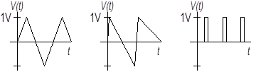
Problem 1.1.14 - Generating Waveforms
|
To gain some familiarity with the scope and function generator, generate the following scope displays for a GSI. Make sure you are able to reproduce the right offsets and voltage levels. (You do not have to write anything.)
Hint: These waveforms are generated with the Ramp and Pulse outputs. To match the depicted waveforms shapes, you will have to adjust the Symmetry and Duty parameters.
|
Problem 1.1.15 - Measurement of DC and AC voltages
(Voltages can be measured using either the scope or the DMM. Connect the scope and DMM in parallel and measure the output voltage of the 5 V power supply using both devices. A good horizontal time-base setting to use is 1ms/div.
a) What are the result and the estimated error of the DMM measurement?
b) What are the result and the estimated reading error of the measurement using the scope?
c) Repeat the measurement for different settings of the V/div knob, and for the other channel of the scope. Are the results consistent with each other and with the DMM measurement?
d) Describe the best scope settings (0V level and V/div) to minimize the reading error.
Problem 1.1.16 - Supply Noise and the Scope AC Setting
|
Keeping the scope connected to the 5V supply, set the scope channel input switch to AC. a) What does this setting do? Expand (increase the sensitivity) the vertical scale. b) What do you see? Describe in detail the AC component of the output. Be sure to explore the full range of the time-scale knob. |
Problem 1.1.17 - RMS Voltages: Calculations
|
The amplitude of an AC signal can be characterized in different ways: by the peak voltage (or amplitude), the peak-to-peak voltage, or the RMS (root-mean-square) voltage. The RMS voltage is particularly useful for measuring the power in a signal; for example, the AC power line voltage, 120V in USA, is an RMS voltage, not an amplitude or peak-to-peak voltage. RMS is calculated by averaging the square root of the average voltage squared: $V_{RMS}=\sqrt{\frac{1}{T_2-T_1}\int^{T_2}_{T_1}dt\,[V(t)]^2},$ where $T_1$and $T_2$ demark the beginning and end of one period of the wavefunction $V(t)$. Derive the coefficients that convert between the amplitude, peak-to-peak voltage, and RMS voltage for a) sine waves, b) triangular waves, and c) square waves. Construct a conversation table showing your results. To verify the coefficients in the conversion tables, feed a 1kHz wave of each type into both the DMM and the scope, using the scope to measure peak and peak-to-peak voltages, and the DMM to measure the RMS voltage. Be sure to put the DMM into the AC/RMS mode. Compare your measured values to the calculated values. (Remember that any quantitative comparison requires consideration of errors on all the measured quantities.) |
Problem 1.1.18 - RMS Voltages: Measurements
Using a sine wave of about 1V p-p (peak-to-peak), vary the frequency of the signal between 10Hz and 10MHz. Measure, as a function of frequency, the RMS voltage of the signal a) using the scope with the input switch on 'DC' (using the conversion constant calculated in Problem 1.1.18), and b) using the DMM. Plot the results. Find the frequency range over which the DMM is accurate (i.e. where the two results agree to within 5%.). Does the DMM perform within specifications? Take at least two measurements per decade (factor of ten) taking a few more per decade at the low and high ends. You should take your data at geometrically rather than arithmetically (i.e. multiplying by a constant each time rather than adding a constant increment) spaced frequencies. Why?
Problem 1.1.19 - Scope AC Settings Distortions
|
Now feed a square-wave into both channels of the scope, with one channel set on 'DC', the other on 'AC'. Compare and sketch the displayed signals for 10Hz, 100Hz and 10kHz square waves, and explain the distortion on the 'AC' channel. Remember these results! A common mistake is to measure the amplitude of low-frequency signals using the ‘AC’ setting of the scope. ‘AC’ on the scope does not mean “use this setting if your signal has an AC component!” Use ‘DC’ unless you have a specific reason to not use it. The only common reason to use the AC setting is to look at a small AC signal riding on top of a large DC. Even then, better results are often obtained by using the DC setting and the vertical level knob to force the trace onto the screen. |
Background: Black Boxes and Thévenin’s Theorem or Thévenin equivalent circuit http://en.wikipedia.org/wiki/Thevenin%27s_theorem
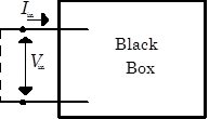 |
Perhaps the simplest general circuit is a box containing some internal circuitry connected to two external leads. Such “thought experiment” boxes are known as black boxes. What can we deduce about the internal circuitry from measurements on the two leads? Let’s assume that there are no frequency dependent elements in the box. The simplest measurements that we can make on the black box are the open-circuit voltage $V_{open}$, and the short-circuit current $I_{short}$. What internal circuit could generate these two parameters? (Open-circuit means that the leads are disconnected from all loads; i.e. no current flows in the leads. Short-circuit means that the leads are connected together with a zero resistance wire; i.e. the leads are “shorted” and there is no voltage drop between the two leads.) |
|
The simplest such circuit is shown to the right. If we set the battery voltage to the measured open-circuit voltage $V=V_{open}$ and set the resistance to $R=V_{open}/I_{short}$, the circuit reproduces the correct open-circuit voltage and short-circuit current. But is it identical to the original circuit for all other conditions? Thévenin proved that it is indeed identical if all the internal components are linear. Linear circuit components are components that obey the linear relation $V=ZI+V_{constant}$, where $Z$is the impedance (similar to the resistance $R$) and is constant. Linear components include resistors, capacitors, inductors, and batteries. The simplified circuit shown at right is called the Thévenin equivalent circuit, and its internal components are called the “Thévenin resistance” and the “Thévenin voltage”. |
 |
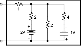
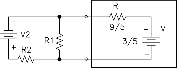
For example, complicated circuit on the left below can be reduced to the Thévenin equivalent circuit on the right below by measuring the left circuit's open circuit voltage, which is $V_{open}=3/5V$ and its short-circuit current, which is $I_{short}=1/3A.$ Thus, the circuit on the right must have an internal battery voltage of $3/5V$ to match the left circuit, and a resistor of $R=V_{open}/I_{short}=9/5\Omega$ to possess the same short circuit current.

What happens if you just have the circuit diagram, not the actual circuit, and can't measure $V_{open}$ and $I_{short}$? Textbooks and Wikipedia describe methods for calculating the Thévenin circuit parameters. While these methods are not very hard, it is more important for you to accept that the reduction can always be done then for you to be actually able to do it.
Thévenin’s theorem would be just a curiosity if it only worked for isolated black boxes. Its power lies in the fact that the Thévenin equivalent circuit behaves exactly like the original circuit when inserted into any external circuit.

Time Dependent Circuits
Circuit analysis is straightforward if all the signals are time independent, i.e. DC. The response of circuit to time dependent (AC) signals like sine waves is more complicated because the response to the signal may not be in phase with the signal, and may depend on frequency. For example, a circuit driven by a voltage source $V=V_1\cos(\omega t)$ might produce an output current phase-shifted by $\phi$, namely $I=I_1\cos(\omega t+\phi)$. We can incorporate such phase shifts into Ohm’s law by allowing the voltages, currents, and resistances to be complex. Thus, $I_1\cos(\omega t+\phi)$ becomes ${\bar I}\exp{j\omega t}$, where ${\bar I}=I_1\exp{j\phi}$. (We use $ j$ instead of $i$ for the $\sqrt{-1}$ to avoid confusion with the symbol for the current.)
Note that in this formalism, we do all our algebra with complex quantities, but, in the end, we measure real quantities in a lab. Consequently we implicitly always take the real part of our solution, e.g. $I={\rm Re}[{{\bar I}\exp{j\omega t}}]$. We can almost always ignore this last step; the one significant exception is in calculating the power in a circuit, where we have to be quite careful.
Since $I$ and $V$ are not necessarily in phase, the resistance can no longer be a pure real quantity. We use a new term for complex resistances: the impedance $Z$. The magnitude of the impedance has much the same function in Ohm’s law (now $V=ZI$), as did the resistance $R$; it determines the relation between the magnitudes of $I$ and $V$. The phase angle of $Z$ determines the phase shift between $I$ and $V$. Note that resistance is redefined to be the real part of the impedance, and the reactance is defined to be the imaginary part of the impedance.
Clearly, a resistor has pure real impedance $Z_R=R$, but the impedance of capacitors and inductors is more complicated; capacitors have impedance $Z_C=1/j\omega C$ and inductors have impedance $Z_L=j\omega L$. Capacitor impedance decreases with frequency, while inductor impedance increases with frequency. Both capacitors and inductors induce 90° phase shifts, but the phase shifts are in opposite directions.
A linear circuit is any circuit that consists only of resistors, capacitors, inductors, voltage sources, and current sources; any linear circuit can be analyzed using the impedance formulas. For example, the familiar parallel and series resistor addition formulas carry over directly; just substitute the capacitative and inductive impedances for R. For example, the impedance of two capacitors in parallel is:
$Z=\frac{Z_{C1}Z_{C2}}{Z_{C1}+Z_{C2}}=\frac{(1/j\omega C_1)(1/j\omega C_2)}{1/j\omega C_1+1/j\omega C_2}=\frac{1}{j\omega (C_1+C2)}$
Analyze any circuit just as you would if all the components were resistors, but keep track of the complex parts, and you will get the right answer. Thévenin circuit reduction works as well, though the Thévenin resistance becomes a complex, frequency dependent impedance.
This is all we need to know about complex impedances for this class. But as physicists we should understand the formal differential equations methods that underlie these simplifications. These theoretical underpinnings can be can be found in most E&M texts.
Large Signal Impedance/Input Impedance
To recapitulate, we can model any linear black box with its Thévenin equivalent. The black box’s input impedance is defined to be the Thévenin impedance Z: the ratio of the open-circuit voltage to the short-circuit current $Z=V_{open}/I_{short}$. The Thévenin impedance $Z$ may be a function of frequency, but it is not (yet) a function of the amplitude of any signal. Such impedances are called “large signal” impedances.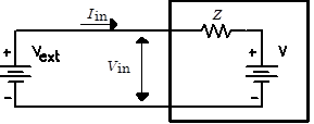
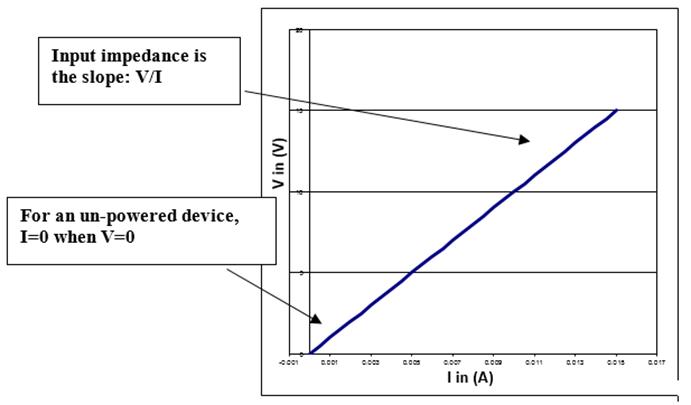
For example, consider the circuit to the right. The input current is related to the input voltage by the equation $I_{in}=(V_{in}-V)/Z$. The proportionality between the current and the input voltage $V_{in}$ is the impedance $Z$, regardless of the amplitude of the external driving voltage $V_{in}=V_{ext}$. In this context, $Z$ is often called the input inpedance.
|
It is often very important to measure the input impedance of a circuit. This can be done by varying $V_{ext}$, but this can be awkward. A more common procedure employs the circuit shown in Fig. 2. (Note that in most situations where we want to know the input impedance, the Thévenin voltage is zero.) To measure $Z_{in}$, we fix the amplitude and frequency of $V_{ext}$ while varying $R$, and measure the corresponding $V_{in}$. For each $R$ and $V_{in}$ we can calculate the corresponding input current $I_{in}=(V_{ext}-V_{in})/R$. The we can plot $V_{in}$ as a function of $I_{in}$. If the circuit is linear, then $Z_{in}=V_{in}/I_{in}$ is just the slope of this curve; in fact, it can be calculated at a single value of $R$: namely, $Z_{in}=[V_{in}/(V_{ext}-V_{in})]R$. |

|
| Figure 2: Input Impedance Measuring Circuit |
In principle, any set of values of $R$ can be used to graph $V_{in}(I_{in})$ and find $Z_{in}$. In practice, values of $R$ that are too large introduce errors because Vin will be too small to measure accurately. Values of $R$ that are too small will introduce errors because calculating the denominator $(V_{ext}-V_{in})$ requires the subtraction of two imprecisely known, but nearly equal numbers. (For example, subtracting 2.1700 from 2.1701 is problematic if both numbers are not known to more than five digits.) Values of $R$ close to $Z_{in}$ generally produce the most accurate results.
If the circuit is not linear (as in later labs), we can find the impedance by taking the slope of the $V_{in}(I_{in})$ curve.
Output Impedance
Output impedance is defined similarly to input impedance, but is used when a black box is putting out a signal, whereas the input impedance is used when we are putting a signal into a black box. In contrast to the input impedance case, we normally assume that the black box of a circuit for which we are attempting to measure the output impedance has some sort of internal power source $V_{th}$. For convenience we also invert the direction of the current: $I_{out}$ is now directed out of the box. (Keep track of which direction goes with which impedance by remembering that input and output impedances are normally positive.)
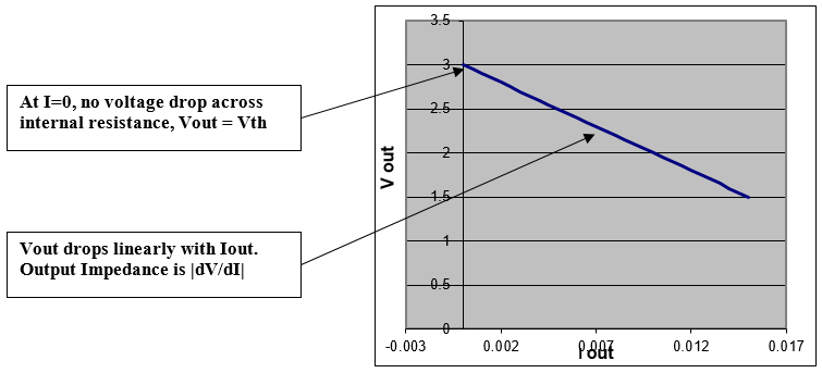
| Output impedance can be measured in roughly the same manner as input input impedances are measured. We hang a resistor off of the output of the circuit as shown in Fig. 3. Then we measure $V_{out}$ as we vary the resistor $R$, infer the output current from $I_{out}=V_{out}/R$, and graph $V_{out}(I_{out})$. These quantities are related by $V_{th}=V_{out}+Z_{out}I_{out}$, so the negative slope of the $V_{out}(I_{out})$graph gives $Z_{out}$. (The internal power source is assumed not to depend on $R$.) More generally, $Z_{out}=-\partial V_{out}/\partial I_{out}$. | 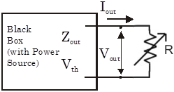
|
| Figure 3: Output Impedance Measuring Circuit |
Remember that there is little actual difference between output and input impedances; which we employ depends on the context. For example, input impedance is defined for the input of a scope, while output impedance is defined for the output of a signal generator.
Note that Problem 1.2.10, given at the end of this writeup, is independent of the other problems in this section. It uses one of two long BNC cables that must be shared between groups. You can (and should) do it at any time the long cables are free.
Problem 1.2.1 - Thévenin Analysis
|
|
| Black Box Connector |
Obtain a black box, and insert the two 9V batteries. Trace out the schematic. Decode the resistor values from the color code by yourself. The Black Box's output connectors are the two 5-wide grey connectors. All 5 spots on one connector are connected (shorted) together.
With the DMM measure the open-circuit voltage $V_{open}$ and the short-circuit current $I_{short}$ across the Black Box output. Draw the Thévenin equivalent circuit and determine the value of the equivalent resistor $R$ by calculating $R=V_{open}/I_{short}$. Now attach a 100$\Omega$ resistor to the output terminals, and measure the output current (through the resistor) and voltage (across the resistor). Repeat for 330$\Omega$, 1$\mathrm{k}\Omega$, 3.3k$\Omega$, 10$\mathrm{k}\Omega$, 33$\mathrm{k}\Omega$ and 100$\mathrm{k}\Omega$ resistors. Plot the measured current against the measured voltage. On the same graph, also plot the output current predicted by the Thévenin circuit as a function of the output voltage, i.e. postulate that the Thévenin circuit is attached to the above resistors, and calculate the output current and voltage. Does the Thévenin circuit predict these voltages accurately? As with all your plots, be sure to label your axes and scales clearly, and don't forget to give the units!
Remove the batteries and short the terminals of each battery holder with a wire. (This replaces the 9V sources with 0V sources.) Use the DMM to measure the resistance between the two terminals. Is it the same as the Thévenin resistance?
Disconnect and remove the 9V batteries when you return the black box.
Note: While you do not have to do so for this problem, it is possible to predict the Thevenin V and Z directly from a schematic for any arbitrary combination of linear circuit elements and ideal voltage supplies. This generally involves solving a system of linear equations. Ask a GSI if you're interested!
Problem 1.2.2 - Pickup Noise
Connect a four-foot BNC cable to the oscilloscope input. Attach a minigrabber clip to the other end, and set the scope to 50mV/div and 4ms/div. Touch the end of the minigrabber signal (red) lead.
a) What is the origin of the signal you see on the scope? Just look at the big signal, ignore, for the time being, ignore any high frequency fuzz.
b) Do you see a signal if you pinch the red insulation rather than the metallic connection of the minigrabber?
c) Now short the minigrabber signal and ground leads together. This makes a "loop antenna". Play with the scope settings. Can you get a clear picture of the fuzz?
d) List some possible sources for the fuzz.
Problem 1.2.3 - Scope Input Impedance
Measure the input impedance of the scope using the circuit given in Fig. 2. Treat the scope as a unknown resistor. Use a frequency of 100Hz, a driving amplitude of 1V p‑p, and several different resistors (for example 0$\Omega$ (a short), 200$\mathrm{k}\Omega$, 470$\mathrm{k}\Omega$, 820$\mathrm{k}\Omega$, 1$\mathrm{M}\Omega$ and 2.2$\mathrm{M}\Omega$, 4.7$\mathrm{M}\Omega$, 10$\mathrm{M}\Omega$, and 20$\mathrm{M}\Omega$.) Record the scope’s input voltage for each resistor, conveniently the scope’s input voltage is displayed on the scope itself.
Plot the input voltage versus input current (determined from Ohm's Law). What is the dependence between input voltage, input current, and impedance? Does the data fit the theory? Determine the input impedance of the oscilloscope from the plot, and make a simple estimate of its uncertainty.
Problem 1.2.4 - Scope Probe Input Impedance
|
Repeat the previous (1.2.3) measurement, but this time connect a scope probe to the oscilloscope and feed the signal generator output into the scope probe. You may need to use higher-valued resistors. Is the input impedance of the scope with the probe higher than with the scope alone? Signals are fed into the scope probe using the minigrabber-like connector at the probe end. Though it is not always necessary, it is generally a good idea to attach the probe's alligator clip to ground. Note that the scope probe attenuates the signal presented to the scope input by a factor of ten. For this exercise, you want to know the size of the signal presented at the probe input, not the scope input. To compensate for the probe attenuation, make sure that you set the "Probe Setup" adjustment on 10X as described in the ScopeProbeAttenuation video on right. An ideal voltage meter would have an infinite input impedance, but this is never obtained in practice. The impedance of the scope without the probe is high, but the probe raises it further. This is always advantageous, but, as mentioned above, the probe also attenuates the signal. This attenuation can be inconvenient when measuring already small signals. In addition to achieving a higher input impedance, scope probes have another advantage; they are better at high frequencies. (You will investigate this phenomenon in the next lab.) Thus, scope probes are primarily used when the signal comes from a high ouput impedance source, or when the signal frequency is high. |
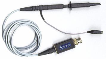 |
| Scope Probe | |
| Scope Probe Attenuation |
Problem 1.2.5 - Output Impedance
Using the circuit given in Fig. 3, determine the output impedance of the signal generator at 1kHz. Measure the output impedance separately for both the 50$\Omega$ and High Z signal generator settings. Use resistors between 2$\Omega$ and 1$\mathrm{k}\Omega$ for your load.
Problem 1.2.6 - RC Circuits: Measurement Techniques
|
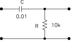
Build the RC circuit shown below. The circuit follows the convention that signals flow left to right; the input terminals are the left and the output terminals are on the right. Note that when units are not explicitly given for a capacitor, the assumed units are $\mu\mathrm{F}$. Before building your circuit, confirm the values of your components using your DMM and the LCR (Inductance-Capacitance-Resistor) meter. The LCR meter can be tricky to use. Ask for help if you’re not sure about how to use it. Capacitors typically have higher tolerances than resistors: generally within about $\pm20\%$ of their nominal value.
Drive the circuit with a 1Vp-p sine wave from the signal generator. Set the signal frequency to 20Hz. You should observe a small signal. Setup Auxillary Triggering between the signal generator and the scope. Configure the scope to measure the peak to peak viltage of the signal. Imrpve the measurement by setting up Averaging. You should obtain a clean, relatively noise-free trace and measurement similar those shown in the adjacent video. Using the Save button on the scope, save an image of the scope screen to a USB thumb drive, and past this image into your notebood. (If you don't have a thumb drive, use your pone to take a picture of the screen. Bring a thumb drive in the future.) |
|
Problem 1.2.7 - RC Circuits: Amplitude Measurements
|
Keep driving the RC circuit from exercise 1.2.6 with a 1V p-p sine waves, and now scan the drive frequency range from 10Hz to 20kHz. Measure the circuit output amplitude as a function of frequency (use 1-2-5-10... frequency steps). Plot $V_{out}/V_{in}$ vs. frequency. (use a log scale for frequency.) Measure the roll-off point, defined as the frequency f where $V_{out}/V_{in}=1/\sqrt{2}$ and mark it on the graph. (Bonus question: why $1/\sqrt{2}$ instead of the more straightforward $1/2$?) Because this circuit sharply attenuates low frequencies, but passes high frequencies unchanged, it is called a high-pass filter. Swapping the positions of the capacitor and resistor results in a low-pass filter in which high frequencies are attenuated. |
|
Problem 1.2.8 - RC Circuits: Phase Measurements
| For the circuit in 1.2.6, measure the phase shift between the input and the output over the same frequency range. Plot this data on the same graph as 1.2.7. Find the frequency or frequencies yielding approximate phase shifts of 0°, 22.5°, 45°, 67.5°, and 90° mark these values on the graph. |
|
Problem 1.2.9 - Analysis
The gain of a circuit is defined to be the ratio of its output to input signal voltage amplitudes. It is usually expressed in decibels:
$G=\bigg|\frac{V_{out}}{V_{in}}\bigg|$ (linear)
$G=20\log_{10}{\bigg|\frac{V_{out}}{V_{in}}\bigg|}$ (dB)
where "dB" is the abbreviation for "decibel". The frequency where G = –3dB (where $|V_{out}/V_{in}|=1/\sqrt{2}$) is known as the "3 dB point" or the "rolloff point". Note that the 3dB point is the point at which the output power (proportional to $V^2$) has gone down by a factor of two.
For the RC circuit analyzed in Sec. 1.2.6-8, plot the measured gain vs. frequency on a log-log scale (most plotting programs have an easy setting for this). Mark the gain axis in dB. This type of plot is sometimes called a Bode Plot. Next, on a new graph, plot the phase shift vs. frequency on a semi-log scale (i.e. with frequency on a log scale and the phase shift on a linear scale). Next, calculate and plot the expected transfer function and phase. (Put the theoretical and experimental curves on the same plots as the measured ones.) Do the theoretical and experimental rolloff points agree?
Problem 1.2.10 - Bandpass Filter
A bandpass filter passes frequencies between high and low rolloff points, and attenuates all other frequencies. It can be constructed from sequential high and low-pass filters. Design, build, and demonstrate a bandpass filter with rolloff points at $f_1$ = 500 Hz and $f_2$ = 10kHz. Choose the impedances such that the first stage is not greatly affected by the loading of the second stage. Take enough measurements to explore your filter's performance and plot your results. (Note that this is not a good way to build a bandpass filter; later in the course, you will build much better circuits.)
Problem 1.2.11 - Cable Propagation Measurements (Note: this exercise can be completed at any point in the lab and does not rely on the previous exercises. We only have two long cables, so you will have to share.)
| a) Connect a BNC T to the scope 1 input. Run a BNC cable from this T to the signal generator, and setup the aux triggering between the signal generator and the scope. Configure the generator to produce isolated pulses like those shown to the right. The pulses should be separated by $2\mu\mathrm{s}$, and be about $60\mathrm{ns}$ long. The pulse amplitude should be 1V, and the pulse baseline should be at ground. To configure the generator, use the Pulse setting (one of the illuminated buttons on the generators's bottom left), set the pulse Duty cycle to 3% (on the Pulse Parameter Menu), and set the High Level and Low Level (on the Amplitude/Level Menu) appropriately. Save the scope image to a thumb drive. | 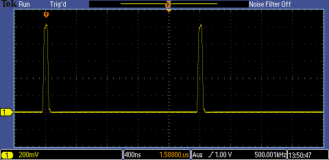
Pulse Train
|
| b) Connect a BNC 50$\Omega$ terminator to the BNC T on scope channel 1. How does the signal change? Save the signal image. Next, remove the terminator and short the scope input signal by connecting a bare wire between the BNC T’s inner and outer conductors. (Use the shortest possible wire.) What do you see on the scope? Save it. |
Input Short |
c) Now disconnect the bare wire and get a standard length (4ft) BNC cable. Connect one end of the cable to the Channel 1 BNC T, and the other end to a T and the scope’s channel 2 input. Henceforth, we will refer to Channel 1 as the "near end" (near to the signal generator) and Channel 2 as the far end. Look at both channels simultaneously. Save the scope signal image.
Now replace the short cable between the near and far ends with a long (at least one hundred feet) BNC cable. Surprised by what you see? Save the image. Connect a $50\Omega$ terminator to the far end T. What happens? Save the signal image. Replace the 50 $\Omega$ terminator with a shorting wire on the far end, and save the signal image. In analogy with the short cable, it should be clear that the case with no extraneous signals (i.e. just one pulse visible at the near end, and one pulse visible at the far end, is more correct. Why, even in this case is the signal at the far end delayed relative to the signal at the near end? (Hint--you have just made your first, approximate, fundamental constant measurement!)
Now consider the cases where there are extraneous signals. When are the extraneously signals at the near end largely upright, and when are some upsidedown?
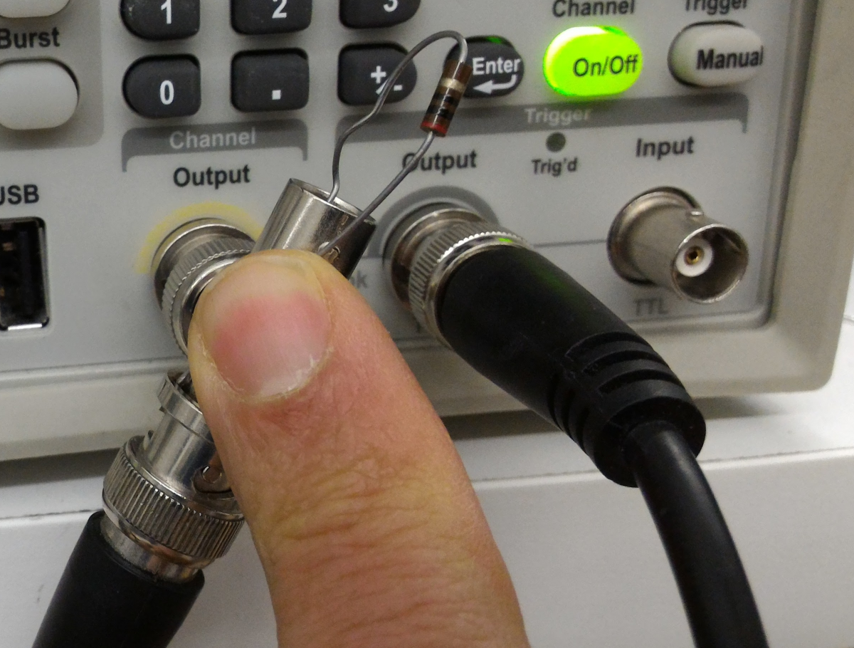
|
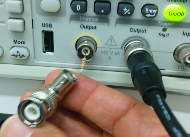
d) Remove any $50\Omega$ terminators or shorts at the far end. Disconect the cable attached to the generator output, and reattach it with an interposed 200 $\Omega$ series resistor. (To accomplish this, use a T as shown in the photo to the right. Notice that the photo does not depict any connection of the outer conductors. This is OK for the purposes of this question, but is not ideal in general. If this bothers you or if you would like a cleaner signal, you may use extra cables and minigrabbers to connect the outer conductors as well). Now what sort of signals do you see with the far end of the long cable (the cable attached to the scope) connected normally, connected with the 50 $\Omega$ terminator, and shorted with the bare wire? Save images of all the signals. Note that the signal generator's intrinsic resistance (called the output impedance, as discussed later in this lab) makes the signal generator's output appear to be like a 50 $\Omega$ resistor connected to ground. |
Series Output Resistor |
|
e) Remove the series resistor, and put a 20 $\Omega$ resistor in parallel with the signal generator output. What do you see on the scope with the far end input connected normally, with a 50 $\Omega$ terminator, and shorted with the bare wire? Save images of all the signals. Try to systemize your results with the 200 $\Omega$ series resistor and the 20 $\Omega$ parallel resistor, as well as the normal case without a resistor. When do you observe only the "expected" signal? When do you get extraneous signals? When are all the extraneous signals largely upright, and when are some upsidedown? Remember that the signal generator's output impedance is 50 $\Omega$ . |
. Parallel Output Resistor |
|
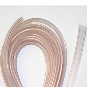
f) The type of coax cable that we use in the 111 lab, and in almost all physics labs, is designated RG-58 cable, and is the most common member of a broad class of cables called 50 $\Omega$ cables. There are many other types of cables; for instance RG-59 cable is representative of the class of 75 $\Omega$ cables, and is widely used in the broadcast industry; the cable industry uses 75 $\Omega$ cable. Cables need not be coax, sometimes they are flat like the cable shown at right. This cable which is a type of 300 $\Omega$ cable, was once commonly used with rooftop TV antennas. Replace the long BNC cable with 50ft of 300 $\Omega$ twin lead cable. What do you need to place at the far end of this cable and at the signal generator to obtain a clean signal (i.e. no extraneous signals)? Just look at the reflected signals; the far end of the cable is awkwardly far away. If you were to attach a 50 $\Omega$ cable at the far end to look at the transmitted signal, the interaction of the 300 $\Omega$ cables and the 50 $\Omega$ cables will lead to confusion. Consequently, just put a resistor at the far end. Hint: the necessary "trick" is relatively obvious at the far end. At the signal generator end you will have to use a series resistor of the right value. The 300$\Omega$ cable is helically wound around a cardboard tube. Please be gentle with it and do not unwind it. Unlike the 50 $\Omega$ coax cables, the 300$\Omega$ twin cable is not well shielded, and nearby wires will interfere. This will ruin the desired effects. The helical winding is designed to keep the wires separate. (It may look like a solenoid, but it is not a solenoid. A solenoid has a single strand of wire in a helical path and produces a fairly uniform field in the center. Our cardboard tube with the twin lead cable is fundamentally different because at any location where a pulse is traveling the local currents are equal in magnitude and oppositely directed.) We are getting off-topic here with this twin lead cable, so don't worry about the details. Someday when you take a course on transmission lines you can study the details. In lecture we will give hints about the resistor values in this problem. |
Twin Lead 300$\Omega$ cable. |
Problem 1.2.12 - Cable Propagation Calculations
The resistors, capacitors, and inductors that we use in this lab are normally physical small compared to the distance traveled by a light (or radio) wave over the relevant circuit time scales, i.e. they are small compared to a wavelength. For example, a sine wave with a frequency of 1kHz has a 300km wavelength, certainly much greater than the size of any component. For high frequency signals, however, wavelengths can be comparable to the size of the components. Circuit analysis under these conditions is much more difficult because the opposite ends of the components experience different signals.
Calculate how long it takes light to travel the length of the long cable you used in Sec. 1.2.10 (Because of the cable's inductance and capacitance, signals propagate on the cable at about 2/3 the speed of light in vacuum.) Does this account for your measurements? Why do you see extra pulses on the near end? And why, depending on what we put at the far end, are the extra pulses sometimes upright, sometimes upside-down, and sometimes not there at all? Hint – Think about what happens when light travels between two media with different indices of refraction.
Analysis:
Problem 1.2.13 - Black Box Output Impedance Calculations
| If the output voltage of a black-box decreases by 20% with a load of 1$\mathrm{k}\Omega$ as compared to the "no-load" output, what is the output impedance of the black-box? |
Problem 1.2.14 - Light Bulb Resistance
| The resistance of a 100W light bulb, as measured with the DMM, is 9$\Omega$. Household power is 110V. Using a power equation, how much power would you expect the light bulb to use? What’s going on here? Is the light bulb a linear circuit component? If not, what accounts for its nonlinearity? Which power number is right? Why is the other power number wrong? |
After completing the lab write up but before turning the lab report in, please fill out the Student Evaluation of the Lab Report.