Lab 2 - Linear Circuits II
University of California at Berkeley
Donald A. Glaser Physics 111A
Instrumentation Laboratory
Lab 2
Linear Circuits II
© 2015 by the Regents of the University of California. All rights reserved.
| The Student Manual, Hayes & Horowitz | Chapter 1, p. 32–60 | |
| The Art of Electronics, Horowitz & Hill |
For the Third Editon of The Art of Electronics: Section 1.4 (Capacitors and AC circuits) Section 1.5 (Inductors and transformers) Section 1.7 (Impedance and reactance) Appendix A (Math Review), page 1097 Here are some older edition references: Chapters 1.06, 1.12-1.24, 5.01-5.02, 5.04-5.05, Appendix H Appendix B (skim) |
|
| Various Books | Readings |
Physics 111-Lab Library Reference Site
Reprints and other information can be found on the Physics 111 Library Site.
Legends: See the Syllabus Web pages for details on introductory Advice next to Glossary.
NOTE: You can check out and keep the portable breadboards, VB-106 or VB-108, from the 111-Lab for yourself ( Only one each please)
In this week’s lab you will continue investigating linear circuits. Fourier analysis, scope probe frequency properties, inductors, resonant circuits, and computer simulations will be studied.
Before coming to class complete this list of tasks:
· Completely read the Lab Write-up
· Answer the pre-lab questions utilizing the references and the write-up
· Perform any circuit calculations use Matlab or anything that can be done outside of lab using RStudio (freeware).
· Plan out how to perform Lab tasks.
Pre-lab
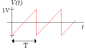
1. Calculate the Fourier coefficients for the ramp waveform shown below:
2. How does the scope probe work?
3. Approximately what is the Q of the KFOG-FM transmitter?
4. Calculate the amplitude response $V_\mathrm{Out}$ of the RLC tank circuit drawn below as a function if the frequency $\omega$ of the current source. Use $\omega_0=1/\sqrt{LC}$ for the resonant frequency (rad/sec). What is the magnitude of the complex amplitude response? Find the very simple expression for the amplitude on resonance.
Next, show that the detuning $\Delta\omega $ is approximately given by $\Delta\omega\approx1/(2RC) $. The detuning, sometimes called the resonance width, is the frequency shift $\Delta\omega=\omega-\omega_0$ that reduces the power in the resistor by a factor of two from the power at resonance. To derive $\Delta\omega\approx1/(2RC) $, make every possible approximation; if you work with the full complex expression for the amplitude, you will very likely get lost. For instance, you only really need consider the denominator. Further, you should approximate the square root; this approximation is valid in the limit that the $Q$ is reasonably large.
Finally, calculate the $Q=\omega_0/\Delta\omega$ of this circuit. This formula for Q is the one we will use when we are speaking in general and/or approximate terms; when we do precise calculations we will put a factor of 2 in the denominator, as will be explained below. The reason for the confusion is that people often talk about the Full Width at Half Max (FWHM) and this is approximately equal to 2 times the Root Mean Square (RMS) width for a Gaussian distribution [Note that an extreme case is the Lorentzian distribution, where the RMS width is infinite and the FWHM is of course finite.] There are also many people simply use the term "the width" for the RMS width.
5. The on-resonant power in the circuit above is proportional to $R$. Find a circuit in which the on-resonant power is inversely proportional to $R$. Note that in both cases, the power is still proportional to $Q$
Background
Fourier Analysis and Repetitive Waveforms
In last week’s lab, we showed how the concept of complex impedances extends our ability to analyze circuits to those driven by pure sinusoidal waveforms. However, our circuits will be frequently driven by waveforms more complicated than pure sinusoids. Fortunately complex impedance analysis is easily extended to include circuits driven by any repetitive waveform by using the fact that any repetitive waveform can be decomposed into a (possibly) infinite series of harmonic sinusoids. The mathematical technique which performs the decomposition is called Fourier Analysis – you should have already studied this technique in your mathematics classes. In summary, any waveform $F(t)$ which is repetitive [has a period $T$ defined such that $F(t+T)=F(t)$ for all $t$] can be synthesized from the infinite sum
$F(t)=\displaystyle\sum_{n=0}^\infty \big[A_n\sin(n\omega_0t)+B_n\cos(n\omega_0t)\big]$
which is the same as
$F(t)=\displaystyle\sum_{n=0}^\infty Re \big[(-j A_n+B_n)\exp(j n\omega_0t)\big]$
where the Fourier coefficients are defined as
| $A_n=\displaystyle\frac{2}{T}\displaystyle\int_0^TF(t)\sin(n\omega_0t)\,dt$ |
 |
| $B_n=\displaystyle\frac{2}{T}\displaystyle\int_0^TF(t)\cos(n\omega_0t)\,dt $ | |
| $B_0=\displaystyle\frac{1}{T}\displaystyle\int_0^TF(t)\,dt $ |
where $\omega_0=2\pi/T$. The formula for $B_n$ is to be used only for nonzero values of n. The lowest order sinusoid ($n=1$) in the infinite sum is called the fundamental; all the other waveforms are referred to as the $n^\mathrm{th}$ harmonic.
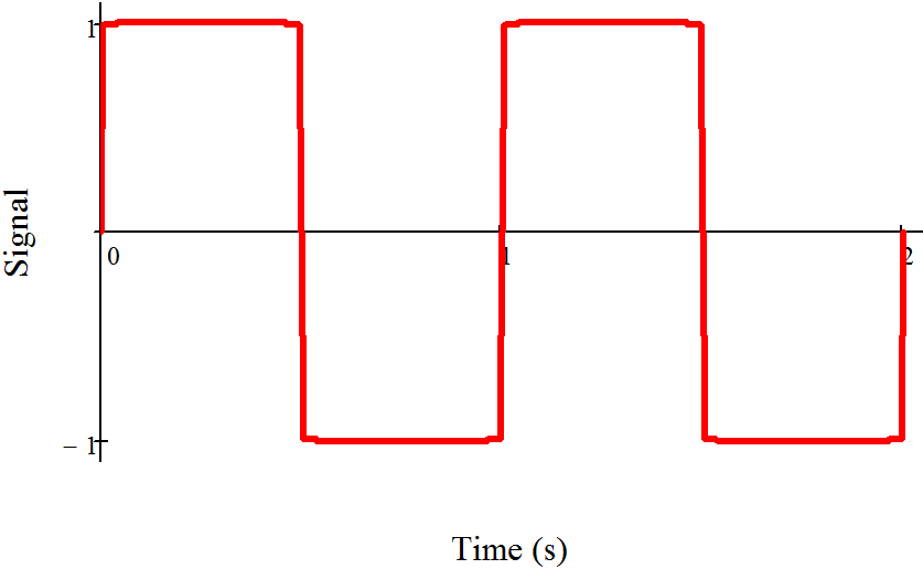
For example, the square wave shown to the right has Fourier coefficients $A_n=4/n\pi$ for $n$ odd, with all other coefficients equal to zero.
The beauty of using Fourier Analysis in circuit analysis is that the response of any linear circuit to a repetitive waveform is the sum of the responses of the circuit to each individual harmonic. Thus a circuit with a transfer function $H(\omega)$, driven by the repetitive waveform $F(t)$, has the output
$\displaystyle\sum_{n=0}^\infty Re \big[(-j A_n+B_n)\exp(j n\omega_0t) \, H(n\omega_0)\big]$
|
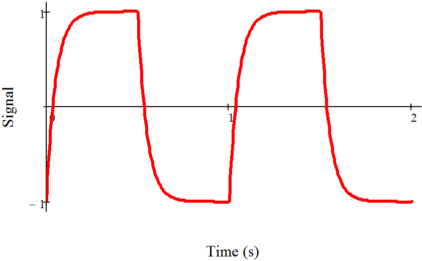
For example, when a 1Hz square wave is passed through a $\tau = 50\mathrm{ms}$ low pass filter [transfer function $H(\omega) = 1/(1+j\omega\tau)$], the calculation is summarized in the table below and the output waveform is shown in the graph to the right. |
 |
|
Harmonic |
Frequency (rad/sec) |
Square Wave Coefficient |
Low Pass Filter Transfer Function |
Output Coefficients |
|
$n$ |
$\omega_n$ |
$A_n$ |
$H(\omega_n)$ |
$A_nH(\omega_n)$ |
|
1 |
6.283 |
1.273 |
0.91-0.286j |
1.159-0.364j |
|
3 |
18.85 |
0.424 |
0.53-0.499j |
0.225-0.212j |
|
5 |
31.416 |
0.255 |
0.288-0.453j |
0.073-0.115j |
|
7 |
43.982 |
0.182 |
0.171-0.377j |
0.031-0.069j |
|
9 |
56.549 |
0.141 |
0.111-0.314j |
0.016-0.044j |
|
11 |
69.115 |
0.116 |
0.077-0.267j |
0.009-0.031j |
|
13 |
81.681 |
0.098 |
0.057-0.231j |
0.005-0.023j |
|
1001 |
6289.468 |
0.0013 |
1.0E-5-3.2E-3j |
1.3E-8+4.0E-6j |
Resonant Circuits
|
Figure 1 |

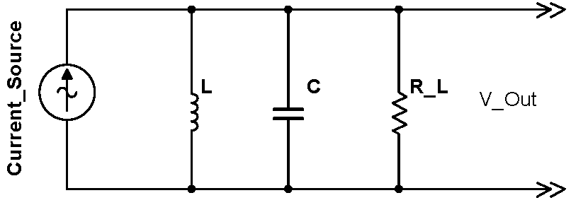
A circuit combining an inductor and capacitor in parallel, sometimes called a tank circuit, will oscillate at the frequency $\omega=\frac{1}{\sqrt{LC}}$ .
Such resonant circuits are frequently used in physics and electronics. They have two primary applications: detecting signals oscillating at a known frequency, and generating signals at a specific frequency. The first application is exemplified by radio tuners which pick out a specific radio station (say at 1MHz) from the enormous selection of available radio stations, and the second is exemplified by the radio station transmitter itself, which must broadcast at a precisely controlled frequency For instance, KFOG-FM’s carrier frequency is allowed to drift only 2kHz (0.002%) from its assigned frequency of 104.5MHz.
Resonant circuits are endlessly analyzed in the course textbooks. Here we will review only a few points:
- Understand the energy flow: the energy sloshes back and forth (at the resonant frequency) between the capacitor (maximum capacitor voltage, no current) and the inductor (maximum current, no voltage across the capacitor.)
- The oscillation amplitude of a resonant circuit will be much higher when driven with a frequency near resonance than when driven off resonance. Thus, resonators will preferentially respond to near resonant signals, and can be used to detect such signals even when these signals are masked by signals at other frequencies.
- Remember that the impedance of an inductor is proportional to j while the impedance of a capacitor is proportional to 1/ j = – j. Both inductors and capacitors induce 90° phase shifts, but in opposite directions. Consequently, their phase shifts are 180° apart from each other. At resonance the magnitudes of the impedances are equal. Add them together and you get zero! Thus the impedance of a series combination of inductors and capacitors is zero, and the impedance of a parallel combination, like that drawn in Fig 1, is infinite.
- Resonating circuits always have some dissipation, either from a deliberately added resistor or from imperfections in the circuit components; typical imperfections include resistance in the inductor windings and dissipation in the inductor core and the capacitor dielectric. The Q of a resonator is a measure of the “quality” of the resonator; the lower the dissipation, the higher the Q. There are several definitions of the Q:
- For a driven resonator, the oscillator resonant frequency $\omega$ divided by twice the de-tuning frequency $\Delta\omega$. The detuning frequency is the driving frequency shift that results in the resonator power amplitude dropping by a factor of two.
- times the number of times the resonator will ring or oscillate after it has been hit with an impulse excitation before the voltage drops to 1/e.
- $2\pi $ times the energy stored in the oscillator divided by the energy dissipated in one cycle.
- Approximately proportional to the amount that the oscillation amplitude peaks up when driven at resonance compared to the amplitude when driven far off resonance. While useful conceptionally, this definition is imprecise because the calculation depends on how far off resonance one chooses.
- Depending on the circuit configuration, various combinations of R, L, and C. Be warned…the Q is sometimes proportional to R, and sometimes to 1/R.
These definitions work best for high Q.
- A common misconception is that the highest possible Q is always best. Very high Q’s are desirable for sources like fixed frequency transmitters, where very pure frequencies are needed. However, high Q’s are not necessarily desirable for transmitters or receivers broadcasting information; information cannot be conveyed by a pure, single frequency wave. The signal has to have a bandwidth $\Delta\omega$ equal to the highest frequency in the signal to be conveyed. Thus, in such applications, circuitry will be designed with resonators that have a Q is approximately equal to $\omega/\Delta\omega$.
For example, radio stations broadcast information around a central base frequency called the carrier frequency. But since they have to transmit information, they actually broadcast in a band surrounding their carrier frequency. The station KFOG-FM, for instance, has a carrier frequency at 104.5MHz, but it actually broadcasts between about 104.450 and 104.550MHz.
Simulations
Numeric computer simulations have revolutionized many fields of physics and electronic design. Today’s astonishingly powerful desktop computers have made simulations a common tool of almost every physicist. Simulations are used in every field: in condensed matter physics, astrophysics, plasma physics, even biophysics. And modern integrated circuits are almost entirely designed with the aid of computer tools and simulations. BUT beware of the allure of simulations. While simulations have their place for analytically intractable problems, an analytic solution is almost always worth a thousand computer simulations. Use them for problems like the band structure of a complicated crystal or to find the attractors in a chaotic system. Don’t use them to solve for the behavior of a simple harmonic oscillator.
That said, in this course you will use computer simulations to study circuits that are, by and large, analytically tractable. Worse yet, all the circuits will be readily constructible on a breadboard. Always trust an experimental result over an analytic result, and trust an analytic result over a simulation. To be fair to theorists, though, remember that this statement was written by an experimentalist. And experimental results are sometimes wrong: witness Opera.
So why are we having you run simulations? Our primary purpose is for you to get a flavor of what computer simulations can do, and how they can be run. In addition, some phenomena like phase shift scaling can be studied more easily with the simulations than in the lab.
|
|
You will be required to simulate a small number of circuits as part of this course. If simulating stimulates you, you can play with many other circuits on your own. The circuits indicated by the computer icon are available in the lab and over the web. You can also design and simulate your own circuits.
The circuit simulator we use is called MultiSim, and is written by National Instruments. MultiSim is based on Spice, a very powerful circuit simulation engine which was developed here at Berkeley in 1973. Spice by itself is almost impossible to use; it requires input in an obscure input format reminiscent of the computer input cards that went out in the 70s. Many commercial companies have incorporated the Spice engine or extensions into commercial products; MultiSim is one such implementation. It has a decent MS Windows front end that mostly hides the native Spice input format, and an adequate back end graphing program that displays the results of your simulations.
These programs are often very expensive; a single seat license for Multisim costs two to four thousand dollars. Competing programs are even more expensive; Altium, a popular program, costs almost ten thousand dollars for a single seat license. Various chip maunfacturers have free simulation software, but typically limit their use to the manufacturers' own components. There are some free limited-functionality simulators not tied to maunfacturers or vendors. Fortunately, we have a site license for Multisim; you may download a free copy from the "My Computer BSC Share" site in the 111-Lab.
The circuit solution can be graphed as a function of time. Such solutions are called transient analyses. Perhaps more useful is MultiSim’s ability to scan the master differential equation over a set of frequencies. The program can then extract some circuit characteristic like the transfer function, and graph it as a function of frequency.
Linear Analysis
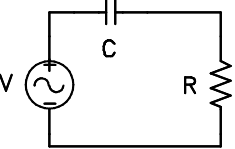
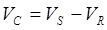
An RC circuit driven by an exponential source turns out to be analytically tractable. By solving the appropriate differential equation, we can prove that the response is exponential, and find the correct multiplicative constant relating the circuit’s output to its input. The first step is to write out what we know from ohm’s law and impedance.
 ,
,  ,
,  ,
, 
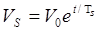
This yields a Differential Equation of the Form: $\frac{dI}{dt}+\frac{I(t)}{RC}=\frac{CV_0}{T_SRC}e^{t/T_s}$
And has the solution $I(t) = \frac{V_0 C}{T_s+RC}e^{t/T_s}$. Now $V_R = I(t)R=\frac{V_0RC}{T_S +RC}e^{t/T_s}$ and $V_R=V_S\left[\frac{RC}{T_S+RC}\right]=V_S\left[\frac{1}{\frac{T_S}{RC}+1}\right]$ .
The point of this discussion is to give a mathematical background and proof-by-example for a common statement in electronics: Linear circuits have linear effects. We know this is true because all signals can be represented with exponentials (typically with complex arguements) and we just proved that an exponential input is still an exponential on the output of a circuit; only the multiplying constant changes. We can also see that the constant is determined by the period or frequency of the signal and the RC (time constant) of the circuit.
In the Lab
 Problem 2.1 - Fourier Analysis
 |
Explore Fourier analysis with the computerized Fourier Synthesizer.[8] Generate square, triangular, and pulse waveforms, and find the effect of small changes to the harmonic amplitudes. Type in and check the coefficients you derived (in the pre-lab questions) for a ramp waveform. Why isn't the Fourier Synthesizer output perfect? |
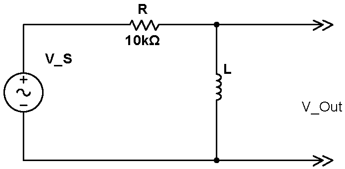
Problem 2.2 - High Pass Filter with Square Wave Drive
| Rebuild the high pass filter that you used in Lab, 1 Part 2. Examine the output from the filter when driven by a square wave. Look at frequencies ranging from 100Hz to 20kHz. Explain your results in terms of Fourier decomposition. | 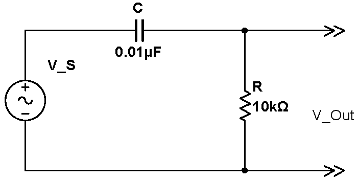 |
Problem 2.3 - Filter Frequency Component Phase
Note how the real-world RC high-pass filter alters the shape of a square wave. Compare this to how high-pass filtering (by turning off the low frequency components) in the Fourier synthesizer alters the shape of the waveform. Why are these different? Hint: think about phase shifts. (There are inteesting connections to causility involved here, which you could explore if you you are curious.)
Problem 2.4 - Low Pass Filter with Square Wave Drive
Rebuild your circuit as a low pass filter, and repeat question 2.2.
Inductors
Inductors are complementary to capacitors; almost any circuit that can be built with a capacitor can, at least in principle, be built with an inductor. In practice, inductors are rare because practical inductors are far less ideal than practical capacitors; practical inductors have resistance and cross turn capacitance. The increased use of integrated circuits has furthered the decline of inductors; while chip capacitors are easy to fabricate on a chip, inductors are almost impossible to fabricate. However, inductors are still important in resonators and transformers.
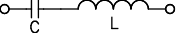
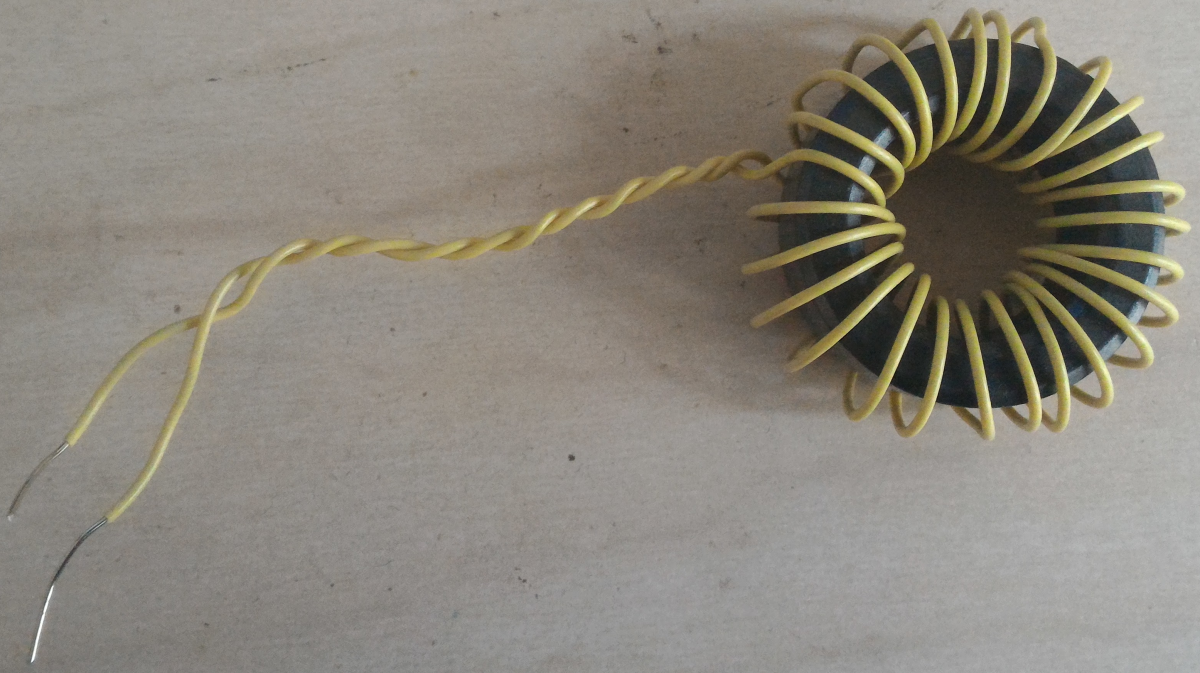
Problem 2.5 - Inductor-based High Pass Filter
|
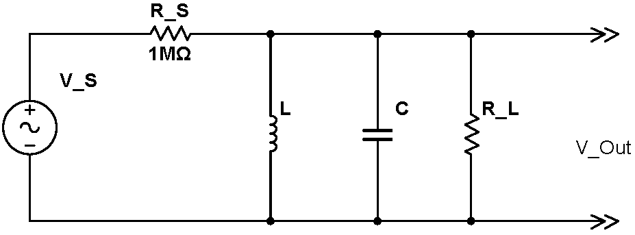
Problem 2.6 - RLC Circuit Resonator
|
Using the inductor that you made for Sec. 2.5, construct the RLC resonator circuit shown at right. Design the circuit to resonate around 10 kHz. What value capacitor should you use? Initially, use a load resistor $R_L=10$k. Set the function generator to produce a 20Vpp voltage. Note that the $R_S=1\,\mathrm{M}\Omega$ resistor isolates the function generator from the resonator circuit. Because the impedance of this RLC circuit is generally low, the function generator, along with $1\,\mathrm{M}\Omega$ resistor, acts as a current source, in this case of $20\mathrm{Vpp}/1\mathrm{M}\Omega \approx 20\mu\mathrm{App}$. Find the resonance by adjusting the signal generator frequency. Is it near your predicted value? Determine the output amplitude as a function of frequency from 1kHz to 100kHz. To fully describe the response, you will probably have to take on the order of 35 measurements. Space your points geometrically, but close together near the resonant peak, and more widely spaced far from resonance. You should be able to see the detailed structure of the resonance peak. Use averaging to make accurate measurement, particularly far from resonance where thje signal is small . Graph your measurements on a Bode plot. From the graph, find the resonance width $\Delta\omega$ ($\omega=\omega_0\pm\Delta\omega$ are the frequencies at which the power in the resistor drops by a factor of two), and calculate the experimental $Q$. For this calculation please include the factor of 2 in the denominator of the formula for Q. See the discussion in prelab question 4. Add the expected theoretical response to your plot. Assume that the voltage source and $R_S$ act like a current souce, so that you can use the formula that you derived in the pre-lab, You can measure $Q$ without taking the entire resonant response curve. Just vary the frequency until you find the resonance, and then measure the peak amplitude response. Then, search for the detuning that reduces the peak response by $\sqrt{2}$. Measure and graph the $Q$ for $R_L$ of 330, 1k, 3.3k, 10k, 33k, and 100k resistors. Using the formula for $Q$ that you derived in the pre-lab, add the predicted $Q$ to your graph. Do the curves agree? Can you explain the descrepancies? |
 |
Transformers
Pacific Gas and Electric provides us with power at ~120V, 60Hz AC. Most electronic circuitry works at far lower voltages: typically ±12V DC for analog circuits and +5V for digital circuits. Transformers are used to lower the wall voltages down to voltages useful for electronics. In the past transformers were also used to change the voltage- current characteristics of signals; however, most such uses are archaic.
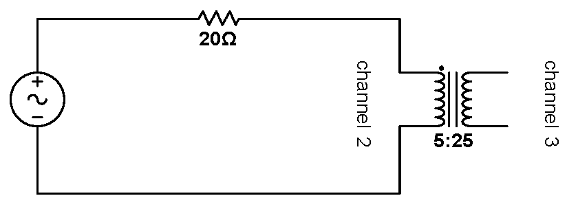
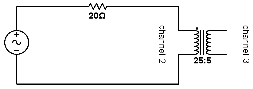
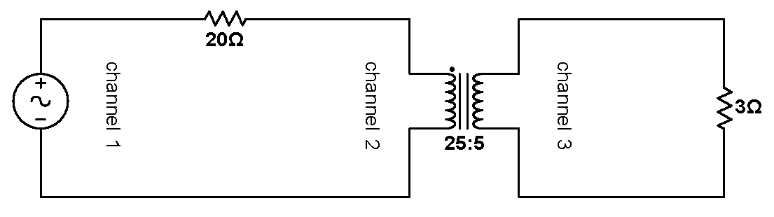
Problem 2.7 - Transformer
|
Construct a 5:1 transformer by winding five additional turns of a second wire around your toroid. Drive the 5-turn winding with a $5\,\mathrm{Vpp}$, $100\,\mathrm{kHz}$ signal. Use a $20\,\Omega$ resistor to isolate the signal generator from the transformer. Set the scope to look at the voltage across both the input (the 5-turn winding is the primary, measured on scope channel 2) and the output (the 25-turn winding is the secondary measured on scope channel 3) of the transformer. What is the voltage ratio? Does this Stepup ratio agree with the predicted value? Now reverse the transformer: drive the 25-turn winding (pirmary) and look at the output on the 5-turn winding (secondary). To make the signals larger, increase the signal generator voltage to $20\,\mathrm{Vpp}$ (the signal generator will have to be on its High Z output). What is the voltage ratio between the input and output windings? Does this Stepdown ratio agree with its predicted value? Now obtain a $3\,\Omega$ resistor and measure and record its resistance with the RLC meter (the resistance of these resistors tends to be off.) Use this $3\,\Omega$ resistor to load the 5-turn transformer output winding. Remeasure the Stepdown ratio. Next attach scope channel 1 to the output of the signal generator. The difference between the voltages on scope channel 1 and 2 is the voltage drop across the $20\,\Omega$ resistor. This difference is small, but can be measured, most easily by using the Math functionality of your scope (see the video at right). Measure the voltage drop across the $20\,\Omega$ resistor, and calculate the current through the 25-turn winding. Then measure the voltage across the $3\,\Omega$ resistor and calculate the current through the 5-turn winding. What is the ratio of these currents? Does this ratio agree with the predicted value? |
Stepup |
|
Stepdown |
|
|
Current Measurment |
|
MultiSim
|
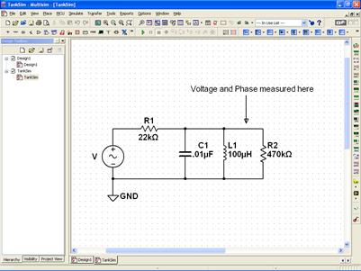
Copy all the MultiSim files from the 111-Lab Network drive to your Desktop or My Documents folder. The first circuit that we will study with MultiSim is the resonator circuit that you constructed in Problem 2.6. Run MultiSim, double click on the TankSim.ms11 after MultiSim opens up, the monitor should display something like the display at the right You will have to change the values of the circuit components to match the values you used for the circuit you constructed in 2.6. You can do this by double clicking on the value. The circle with a squiggle |
 |
|
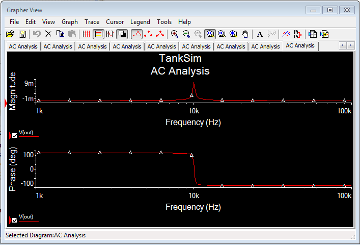
Begin by undertaking an "AC Analysis": finding the response of the circuit as the frequency of the sine wave source is varied. Follow the menus Simulate→ Analyses and Simulation → AC Sweep. On the first tab, adjust the frequencies for a scan between $1\,\mathrm{kHz}$ and $100\,\mathrm{kHz}$. Then press the Simulate button. A new window resembling the one shown at right will pop up which will display the results of your simulation. Both the transfer function (the voltage at the voltage probe vs. frequency) and the phase are displayed on the graph. Since the y-axis for these two curves are so different, the curves need to be plotted on two different graphs. This is easy to do manually, but has already been set up for you. The upper graph is the transfer function, and the lower is the phase curve. Note the both curves plot data from the signal "V(out)". In Multisim/Spice lingo, this means that the plots analyse the voltage on the wire designated "out". Click on the wire pointed to by the arrow in the schematic to see the wire designation. Then go back to the AC Analysis popop and goto the tab "Output" to see where "out" was selected to be ploted. |
 |
 is the pictorial representation of a sine wave source.
 Problem 2.8 - Multisim Tank Simulations (Note: Never save up your signature requests; do them one at a time as they are needed. They are an opportunity for deeper exploration and reinforcement of foundations, and this process does not work well when compressed into one chunk.)
|
Go back to the schematic. Play with the component values and rerun the simulation. How do you increase the Q? Does the phase shift make sense? It will help you to see the change in Q if you increase the number of samples from 10 to 100. |
The response of passive circuits to sine waves is generally easy to analyze using complex impedances. The response of passive circuits to non-sinusoidal signals is more difficult to analyze. As was discussed earlier, repetitive signals can be analyzed by breaking down the signal into its frequency components (via Fourier Analysis), but the response to non-repetitive signals requires the direct solution of the system differential equations.
Problem 2.9 - Multisim Transient Simulations
|
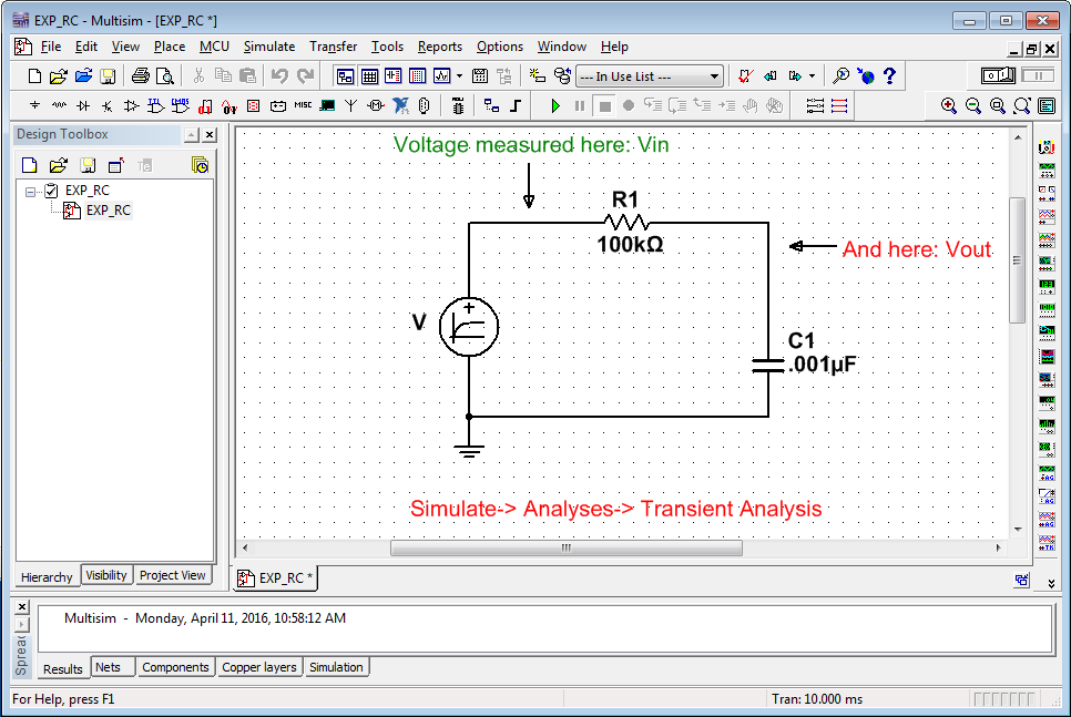
One such non-repetitive signal is an exponential voltage. Go back to MultiSim and use the Open tab item to load the Exp_RC schematic. The circuit contains an exponential source and two voltage markers: the first records the signal output by the source itself, and the second records the response. Analyze the circuit using Transient analysis. Note that aside from a small transient in the beginning, the response to the exponential input appears to be an exponential with the same time constant. Play with the circuit components. Is the response still exponential? An RC circuit driven by an exponential source turns out to be analytically tractable. |
|
More on probes
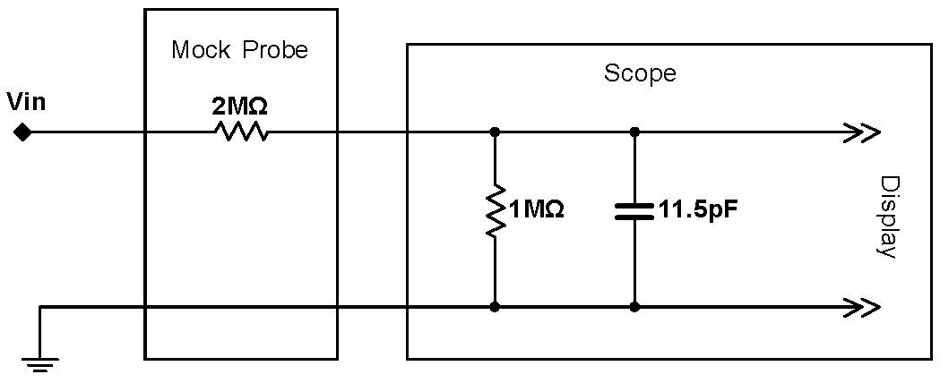
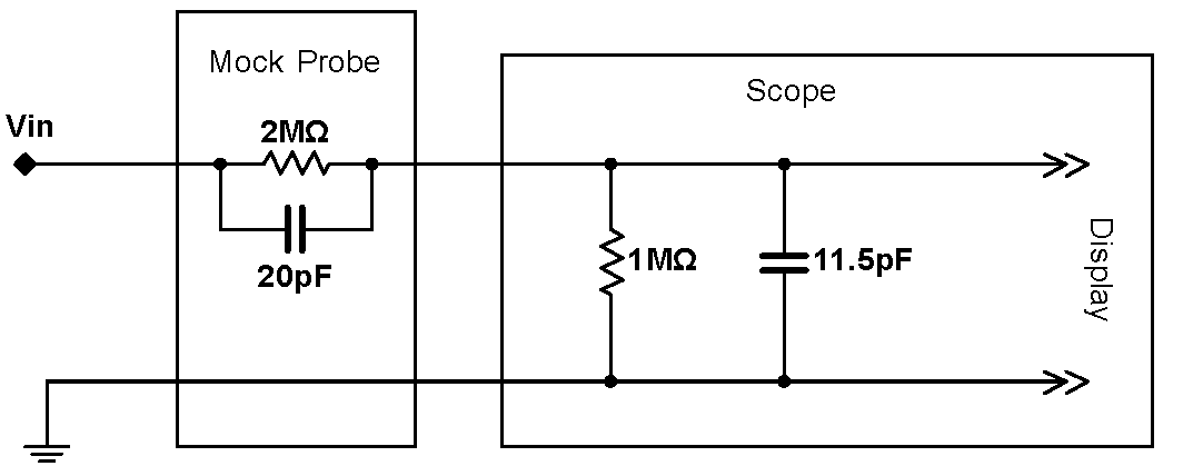
As you studied in last week’s lab, the scope probe increases the input impedance of the scope by a factor of ten – at the expense of attenuating the signal by a factor of ten. The input impedance of the scope by itself is $1\,\mathrm{M}\Omega$ in parallel with $11.5\,\mathrm{pF}$. (The impedance is written on the face of the scope next to the BNC input jack.) The scope probe contains a resistor, which, in conjunction with the scope input resistance, forms a voltage divider.
Problem 2.10 - Resistive Mock Probe-DC Measurements
|
Build the mock probe shown at right hook it up to the scope. (We do not stock 2M resistors; synthesize one out of the components we do stock. Obviously you do not have to build the internal scope circuit. Start with the mock probe disconnected from the scope. Put $V_\mathrm{in}=24\,\mathrm{V}$ across the mock probe input and ground. With the DMM, measure the voltage at the input and output of the mock probe. Why aren’t the two measurements the same? Connect the mock probe to the scope with a short coax cable and mini-grabbers. (Don’t use the real scope probe.) Use the DMM to repeat the measurement of the voltage before and after the mock probe, but now with the scope attached. Is this set of measurements the same as the last set? With which DMM measurement does the scope display agree? Explain all these results. |
 |
Problem 2.11 - Resistive Mock Probe-AC Measurements
Connect the mock probe to the signal generator, and set it to output sine waves. Scan the signal generator frequency from 10Hz to 1MHz. Plot the response, using the scope to measure the size of the signal, as a function of frequency. What are the circuit’s measured and calculated rolloff points? Does the circuit behave like a low-pass filter? Now draw some typical waveforms for square wave inputs.
Hint-The capacitance of the cable connecting the mock probe to the scope is important to the behavior of this circuit. You may wish to measure this capacitance.
Problem 2.12 - Balanced Mock Probe
|
Since a scope is supposed to display an undistorted representation of the input wave, the unintentional low pass filter behavior of the mock probe is not tolerable. Real scope probes are “compensated” to remove the undesired probe low-pass filter. Build the compensated mock probe shown at right. Scan the frequency range again. Does the compensated mock probe work better, especially for square waves? Now increase the value of the $20\,\mathrm{pF}$ capacitor. Is the compensation better? Tweak the capacitor value until you get the best results. What value works best? Is it possible to remove all the frequency dependence in the mock probe? How? Can you calculate this best capacitance value? How? |
 |
After completing the lab write up but before turning the lab report in, please fill out the Student Evaluation of the Lab Report.